Measuring and utilizing temporal network dissimilarity

Temporal dissimilarity characterization

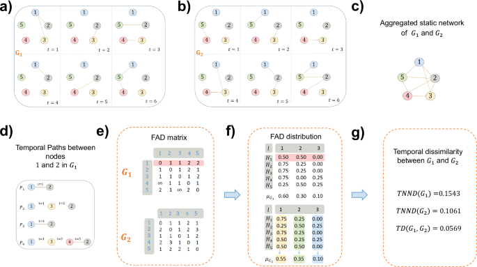
For a given temporal network G = (V, E) in a time window [0, T], V represents the node set, and E = {(i, j, t), t ∈ [0, T], i, j ∈ V} is the contact set. An element (i, j, t) indicates that there is a contact between nodes i and j at time step t. The number of nodes and temporal edges is given by N and C, respectively. The aggregated static network G^s of a temporal network G is the graph with the same node set and an edge between all pairs of nodes that have at least one temporal edge in E. The number of edges in the aggregated network G^s is denoted by M. In Fig. 1a−c, we show examples of two temporal networks with five nodes and six timestamps, i.e., G₁ and G₂, and its corresponding aggregated static network.

A temporal path P in G is a node sequence \(P={\{{i}_{\nu }\}}_{\nu = 1}^{n+1}\), where (i_ν, i_ν+1, t) ∈ E for all ν ∈ [1, n]. The length of P, l(P), is defined as the number of contacts in the path. In this work, we shall base our temporal dissimilarity on the concept of first arrival paths, which can capture both topological and temporal proximity between nodes and has been shown to be an effective way to extract temporal network topology²⁸. Given two nodes i_s and i_g, we suppose the first time when i_s appears is t_s. The first arrival path between nodes i_s and i_g is the temporal path from i_s starting at t_s that reaches i_g the earliest. Meanwhile, we adopt the first arrival distance (FAD) as the length of the first arrival path between two nodes. The temporal paths between nodes 1 and 2 in G₁ are shown in Fig. 1d, i.e., P₁, ⋯  , P₄. According to the definition of the first arrival path, we can obtain that P₁ is the first arrival path between nodes 1 and 2, and thus the FAD value between them is l(P₁) = 1.

We define the FAD distribution of node i as H_i = {h_i(q)}, where h_i(q) is the fraction of nodes with an FAD of q from i. There is exactly one node with an FAD of 0 to node i, namely, node i itself, as it can reach itself in zero time. Consequently, we have h_i(0) = 1/N for every node i. To construct the FAD distribution for each node, we consider q starting from 1. We use \({l}_{\max }\) to denote the maximal FAD among all first arrival paths in a temporal network. If every node pair is reachable through a first arrival path in a temporal network, the dimension of H_i is \(1\times {l}_{\max }\). If there are node pairs in a network that are not reachable, we define the maximal FAD between reachable node pairs as \({l}_{\max }\) and the infinite FAD is defined as \({l}_{\max }+1\). In this case, the dimension of H_i is \(1\times ({l}_{\max }+1)\). The node specific FAD distribution H_i contains the connectivity heterogeneity of node i. Subsequently, we adopt the Jensen-Shannon divergence to characterize the connectivity heterogeneity of a temporal network based on FAD. The temporal network node dispersion (TNND) reads:

where \(J({H}_{1},{H}_{2},\cdots \,,{H}_{N})=\frac{1}{N}{\sum }_{i,q}{h}_{i}(q)\log ({h}_{i}(q)/{u}_{q})\) is the Jensen-Shannon divergence²⁹. The term \({\mu }_{q}=\frac{1}{N}\mathop{\sum }_{i = 1}^{N}{h}_{i}(q)\) is the average over {h₁(q), h₂(q), ⋯  , h_N(q)}. It represents the fraction of source-destination node pairs with FAD q. The average FAD distribution of a network, i.e., the probability distribution of the FAD of a random source destination pair, is given by μ = {μ₁, μ₂, ⋯  , μ_k, ⋯  }. The dimension of μ is either \(1\times {l}_{\max }\) or \(1\times ({l}_{\max }+1)\). Generally, a larger TNND implies higher connection diversity among the nodes.

Finally, for two given networks G₁ and G₂, their temporal dissimilarity, TD(G₁, G₂), reads

where TNND(G₁) and TNND(G₂) represent the temporal network node dispersion, and \({\mu }_{{G}_{1}}\) and \({\mu }_{{G}_{2}}\) are the average FAD distribution of G₁ and G₂, respectively. And ω₁, ω₂ ∈ [0, 1] (satisfying ω₁ + ω₂ = 1) are tunable parameters to measure the contribution of the average FAD distribution and TNND difference, respectively. For the sake of simplification, we use ω₁ = ω₂ = 0.5 in the following analyses unless otherwise specified. Generally, TD falls in [0, 1] and the larger TD is, the more dissimilar the networks will be. For the extreme cases, TD = 1 suggests the two networks are completely different from each other, and vice versa for TD = 0. The detailed procedure of computing the dissimilarity between two exampled temporal networks G₁ (Fig. 1a) and G₂ (Fig. 1b) is shown in Fig. 1e–g. For the two temporal networks, G₁ and G₂, which have the same number of nodes and timestamps, the dissimilarity between them, denoted as TD(G₁, G₂) = 0.0569, indicates a relatively similar temporal structure. However, the dissimilarity value between them is zero based on static network comparison methods because they share the identical aggregated static network structure (Fig. 1c). Therefore, it is of vital importance and urgent necessity to consider network temporality when conducting the comparisons. Regarding computational complexity, we observe that the algorithm’s primary computational cost arises from calculating the first arrival paths between nodes, with a complexity of O(T ⋅ (C + N)).

Comparisons on synthetic temporal networks

To verify the validity of the temporal dissimilarity (TD) metric, we perform comparisons on temporal synthetic networks. The objective is to explore whether the temporal dissimilarity could distinguish synthetic networks with different parameters/properties. The activity driven model³⁰ (see Methods) is used to generate a collection of temporal networks \(G(F(a),m)={\{{G}^{t}\}}_{t = 0}^{T}\) via the tunable function F(a) and parameter m. The function F(a) controls the node activity distribution, and m determines the number of contacts that every active node releases at each discrete time step t. Larger m shall result in a temporal network with more contacts. The distribution of F(a) determines the heterogeneity of activation rates of nodes. In this work, we select two representative types of activity distribution, i.e., (i) the uniform distribution \(F(a)=1/{a}_{\max }\), for \(0\le a\le {a}_{\max }\le 1,\) where a is the active rate of a node and here we choose to use \({a}_{\max }=1\), and (ii) the power-law distribution F(a) = (r − 1)a^−r, where r > 2, 0 < a < 1.

Figure 2a shows the comparison results on synthetic temporal networks generated by the uniform activity distribution for different values of m. It indicates that the temporal dissimilarity tends to be small for the networks generated with similar m, suggesting that networks generated with similar m would be more akin to each other and vice versa. Comparatively, Fig. 2b shows the temporal dissimilarities of temporal networks generated by different heterogeneity parameters r. It shows that the temporal dissimilarity between temporal networks with closer r are inclined to be smaller, suggesting that networks with closer r tend to be similar. Here, the network size N is 300, and the time window size T is 30,000. We can also see similar patterns for different network sizes, time window sizes, as well as other parameters (see Figs. S1−S6 in Supplementary Note 1).

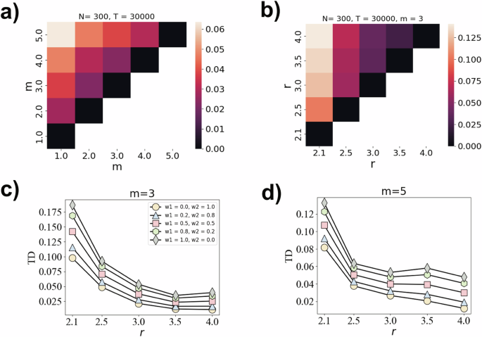
a Temporal dissimilarity between synthetic networks generated by the activity driven model with node activity following the uniform distribution and different m. b Temporal dissimilarity TD between synthetic networks generated by the activity driven model with node activity following the power-law distribution and different r. Here, we set m = 3. Temporal dissimilarity TD between networks generated by the uniform activity distribution and those generated by a power-law activity distribution as a function of r when m is set as 3 and 5 for (c, d), respectively. Different curves indicate we choose different combinations of ω₁ and ω₂ for the calculation of temporal dissimilarity values. Here, each dissimilarity value in every sub-figure is the averaged over 100 realizations. The network size and time scale are set as N = 300, T = 30,000, respectively.

In addition to the analysis in the main text, we compare the temporal dissimilarities between networks derived from uniform and power-law distributions in Fig. 2c, d and also Figs. S7−S9 in Supplementary Note 1. It shows that networks generated by the power-law activity distribution with a higher r are more similar to those generated by the uniform activity distribution. This is because a higher r can result in networks with more homogeneous activity distribution, hence are more similar to the networks generated by uniform activity distribution. These observations in synthetic networks suggest TD to be a powerful index to discriminate the synthetic temporal networks. Meanwhile, the different curves in the figures represent various combinations of ω₁ and ω₂, all of which exhibit similar trends: as r increases, networks generated by a power-law activity distribution become increasingly similar to those generated by a uniform activity distribution. This suggests that the dissimilarity between temporal networks is not significantly affected by the choice of weights, aligning with findings by Schieber et al.²⁶ in their comparison of static networks. Consequently, we adopt ω₁ = ω₂ = 0.5 for most of the experiments.

Comparisons on real-world temporal networks

Here, we introduce 17 representative temporal networks^{31,32,33,34,35,36,37,38}, including five email networks and 12 physical contact networks, to further validate the effectiveness of the proposed method (for details of datasets (Table 1), see Methods). We begin by comparing a temporal network with its aggregated static network. Given a static network, different from the temporal network, we alternatively use the shortest path distance distribution (\({H}_{i}^{s}=\{{h}_{i}^{s}(q)\}\), where \({h}_{i}^{s}(q)\) is denoted as the fraction of nodes that connect to i at shortest path distance q instead of FAD distribution. We then substitute the FAD distribution (H_i) by shortest path distance distribution (\({H}_{i}^{s}\)) in Eq. (1) for the aggregated static network, and then update Eq. (2) accordingly (see Supplementary Note 2 for details).

The resulting dissimilarity between an empirical temporal network and its aggregated static network is shown in Fig. 3a. The nonzero value of the dissimilarity between a temporal network and its static counterpart suggests that insights and regularities may be overlooked when using a static network to address time-varying interactions, particularly if the rich temporal information is ignored.

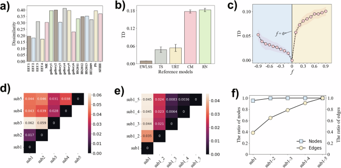
a Dissimilarity between a temporal network and its aggregated static network. b Temporal dissimilarity between the original data and the temporal networks derived from null models. c Temporal dissimilarity between the original and perturbed temporal networks. f denotes the fraction of contacts added (f  > 0) or deleted (f < 0) from the original temporal network (f = 0). Each data point is averaged over 100 realizations. d, e Temporal dissimilarity between different daily divided sub-networks, e.g., sub1 and sub2 represent the temporal sub-networks of the first and second day, respectively. sub1-2 represents the cumulative temporal sub-network for the first two days. f The ratio of nodes and edges of different sub-networks. b−f show comparisons on HS2013, for more results of other networks, see Figs. S11−S13 in Supplementary Note 2.

Comparisons based on temporal null models

We compare each of the empirical temporal networks with their null models^39,40,41, which are obtained by specific reshuffled methods (see Methods). For each null model, topological and temporal correlations are in various degrees of destruction (Table 2). For EWLSS, TS and URT, all topological correlations are preserved, while the temporal correlations are destroyed to different extents. For CM and RN, the temporal and topological correlations are both eliminated in varying degrees. Take HS2013 as an example, Fig. 3b shows that the temporal dissimilarities between the original temporal network and the null models are very small for EWLSS, while the dissimilarities are much larger for TS, URT, CM and RN. It can be found that, although TS only eliminates one more number of properties than EWLSS, it shall lead to higher dissimilarity as it destroys the temporal information (sorted sequence list on each link) other than static topology correlation (weight). Comparatively, even though RN discards the most number of properties, the resulting network does not show significantly different from that derived by CM, suggesting that degree-degree correlation may not be a primary factor in a time-varying environment. Similar patterns can also be found for other datasets in Fig. S11 in Supplementary Note 2.

Comparisons based on network perturbation and evolution

We then assess the discriminative ability of the proposed measure by network perturbation method. That is to say, for a given temporal network, we randomly add or delete a fraction of contacts (f) and then compare the differences. Figure 3c shows the temporal dissimilarity between the original data and gradually perturbed network for HS2013. The negative f corresponds to the deletion process, and vice versa. Large f indicates that more contacts are added (f > 0) or deleted (f  < 0), resulting in larger differences with respect to the original network (f = 0). Note that, for networks with many contacts (large C/N in Table 1), the disparity will even be reduced rather than increased, when adding new contacts (see Fig. S12 in Supplementary Note 2), suggesting that the ceiling effect⁴² of time-varying interactions governs the structural differences of temporal networks.

Furthermore, we examine the temporal dissimilarity from the perspective of network evolution. We divide a temporal network into sub-networks according to the time order of contacts. Take HS2013 for instance, we separate it into five distinct sub-networks where each contains all the contacts in one single day as the observation window is five days. We then use sub1 and sub2 to respectively represent the temporal sub-networks of the first and second day, and sub1-2 to represent the temporal sub-network of the first two days. Similar symbols are also described for other sub-networks. Figure 3d shows that, in general, sub-networks that are closer in time are more similar to each other, e.g., the temporal dissimilarity between sub1 and sub2 (TD_sub1,sub2) is much smaller than those between sub1 and others. This is further enhanced in Fig. 3e that a sub-network that forms earlier is quite different from the whole temporal network (sub1-5) which cumulatively considers all the contacts. It is worth noting that, the short-term temporal dissimilarities (TD_sub1,sub3 = 0.062 and TD_sub2,sub3 = 0.059) are relatively high, indicating that temporal interactions have undergone subtle but noticeable changes in the short run. Figure 3f shows that, although the number of nodes (N) are the same in sub1-4 and sub1-5, the number of links (M) are still slightly different with each other, which can be further captured by our proposed temporal dissimilarity mesure (TD_{sub1-4,sub1-5} = 0.0036 in Fig. 3e).

Applications of temporal network comparison

Temporal network classification

In general, the 17 empirical temporal networks used in this work can be classified into four categories according to the contact type and venues where they were recorded (see Table 1). We first construct a dissimilarity matrix where each element represents the value of temporal dissimilarity of the corresponding two temporal networks (for the full matrix, see Table S1 in Supplementary Note 2). We then adopt multidimensional scaling map⁴³ to show the distance between them in a geometric space (Fig. 4a). It shows that the four categories are spontaneously clustered into two major regions, upper right and lower left (gray shadow). In general, networks from the same category are more likely to be clustered geometrically in the two-dimensional space, except for EEU3 and ME, two essential email networks yet now are situated in the left corner with those of schools and conferences. To obtain a deep understanding, we further study the topological and temporal properties, including (i) link density; (ii) average node degree in the corresponding static networks; (iii) coefficient of variation of the node lifespan CV(Δt), defined as the δ_Δt/ξ_Δt where Δt is the time difference of a node’s first and last occurrence, δ and ξ are respectively the standard deviation and mean; (iv) fraction of reachable node pairs via temporal paths (\(\tilde{R}=\frac{R}{N(N-1)}\), where R is the number of reachable node pairs and N is the number of nodes); and (v) fraction of nodes \({\tilde{N}}_{p}\) in an evolutionary time window [0, p*T], where p ∈ [0, 1]. Results in Fig. 4b−e show that the networks in the same region (gray shadowed or not) in Fig. 4a tend to have similar topological and temporal properties. It is observed that networks clustered in the upper region of Fig. 4a show low link density, average degree, \(\tilde{R}\) but high CV(Δt), and vice versa for lower region (gray shadowed) in Fig. 4a. It also clearly shows that EEU3 and ME have similar topological and temporal properties with those of schools and conferences, which is additionally demonstrated by the evolutionary process of \({\tilde{N}}_{p}\) in Fig. 4f. This suggests that those two virtually connected data may have coincident interaction patterns with the physical contact networks.

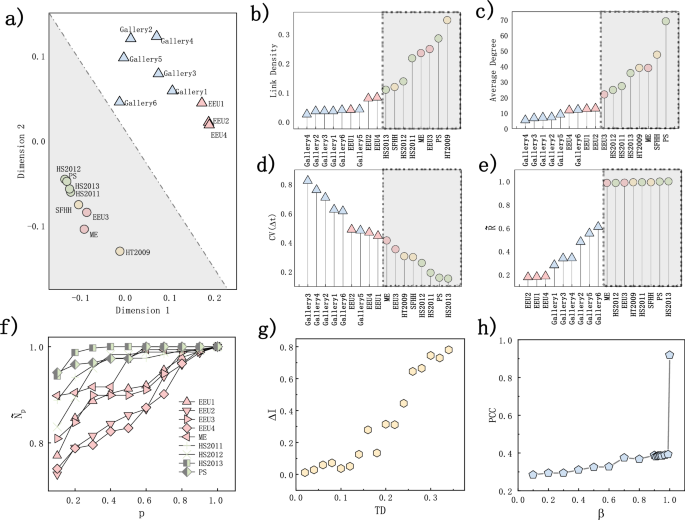
a Multidimensional scaling map of temporal dissimilarity between 17 empirical temporal networks. The colors represent different categories of networks in Table 1. b−e Topological and temporal properties of every empirical temporal network. Gray shadows indicate the same networks at the lower left corner in (a). Link density (b) and average node degree (c) of the aggregated static networks. Coefficient of variation of node lifespan (d) and fraction of reachable node pairs via temporal paths (e) for each temporal network. f The fraction of nodes as the function of network evolution (p). g Spreadability differences as the function of temporal dissimilarity between 17 temporal networks. h Pearson correlation between spreadability differences and temporal dissimilarity as the function of infection probability β.

Temporal network spreadability

The spreading process is one of the most important dynamics of complex networks⁴⁴. Here, we conduct the Susceptible-Infected (SI) spreading process in temporal networks⁴⁵. Initially, an arbitrary node i is randomly chosen as the infected seed (I-state), and all the remaining nodes are set as the susceptible individuals (S-state). The subsequent spreading process shall follow the time step of the contacts. That is to say, at every time step t ∈ [0, T], an I-state node will only infect its neighbors through the temporal contacts exactly existing at t with infection probability β. The spreading process comes to the end at time step T. The fraction of final infected nodes is averaged by setting every node as the seed: \(\langle I\rangle =\frac{1}{N}{{{\Sigma }}}_{i = 1}^{N}{I}_{i}\), where I_i is the final fraction of infected nodes by setting i as the seed. As a consequence, the spreadability difference can be immediately obtained as ΔI = ∣〈I_G1〉 − 〈I_G2〉∣, where 〈I_G1〉 and 〈I_G1〉 are respectively the average fraction of final infected nodes of two temporal networks G₁ and G₂. Figure 4g shows the correlation between ΔI and temporal dissimilarity for every two temporal networks for β = 1. The Pearson correlation coefficient (PCC) is high at 0.919 (p < 0.0001). That is, in time-varying interaction structures, networks with close temporal dissimilarity tend to exhibit similar spreadability when the spreading probability β is equal to 1. Figure 4h further demonstrates that such correlation is becoming more and more obvious as β increases. Actually, when β = 1, the SI spreading process becomes deterministic, while for β < 1, the process is stochastic. Specifically, when β = 1, an infected node will infect all its neighboring nodes at each time step. Consequently, the SI spreading tree for β = 1 is identical to the first arrival tree when a given node is designated as the seed or source, as illustrated in Fig. S16 of Supplementary Note 2. In contrast, for β < 1, the spreading trees differ significantly from the first arrival tree, leading to a relatively lower correlation for β < 1, as shown in Fig. 4h. Despite the SI model, we also evaluate our method’s performance on other diffusion processes, such as the Linear Threshold (LT) model, within temporal networks. Figure S15 in Supplementary Note 2 presents the PCC values between diffusion differences using the LT model and temporal network dissimilarity across various time resolutions. All PCC values exceed 0.5, indicating a strong correlation.