A neural network for modeling human concept formation, understanding and communication

Hierarchical gating of CATS Net

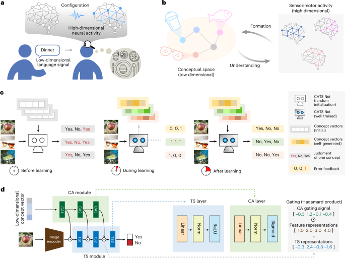
In a concept-abstraction task on an image dataset, we use a 20-dimension real-valued vector to present each category. This dimension was selected from a tested range of 10, 20, 100, as it offered the optimal trade-off between compression efficiency and representational capacity (Supplementary Fig. 1a). The compactness of this vector space, compared with the high-dimensional parameter space of the neural network, reflects the highly compressed nature of the concepts. The model’s pipeline begins with a pretrained ResNet50 backbone¹⁶, chosen over Vision Transformer¹⁷ for its computational efficiency after observing similar performance from both (we use official IMAGENET1K_V1 weights from for both backbones). The extracted 2,048-dimension features are then fed into the TS module. This module is a 3-layer perceptron ([2,048-100-100-2]) with batch normalization and rectified linear unit (ReLU) activation. The 3-layer architecture was adopted for its demonstrated robustness, as our tests with 1, 3 and 5 layers all yielded comparable performance (Supplementary Fig. 1a). To match this structure, the CA module is also a 3-layer perceptron ([20-2,048-100-100]), which takes the 20-dimension concept vector as input and uses the Sigmoid function \(\sigma (x)=\frac{1+ ^{-x}}\) to generate controlling signals between 0 and 1. The output layer of the TS module consists of two neurons for ‘Yes’ (0, 1) and ‘No’ (1, 0) classification, optimized using a cross-entropy loss.

Consider a multi-layer perception of L + 1 layers, indexed by l = 0, ⋯, L with l = 0 and l = L being the input and output layers. Let \({W}_{l}^{\mathrm{TS}}\) be the connection weight between the (l−1)th layer and lth layer in the TS module, and \({W}_{l}^{\mathrm{CA}}\) for the CA module. x_l−1 denotes the input of the connections \({W}_{l}^{\mathrm{TS}}\) and c_l−1 denotes the input of the connections \({W}_{l}^{\mathrm{CA}}\). o_l denotes the output of the connections \({W}_{l}^{\mathrm{TS}}\) and g_l denotes the output of the connections \({W}_{l}^{\mathrm{CA}}\). It is clear that the dimension of feature extractor output is the same with the x₀ and the dimension of concept vector is with c₀. For the CA module, after applying normalization and activation to the g_l, it will be the input c_l for weight \({W}_{l+1}^{\mathrm{CA}}\).

The CA module does not need to directly modulate the feature extractor, because it is possible to utilize gating signals in a much easier way to modulate the processing of the feature extractor. The dimensions of \({{\bf{x}}}_{l-1}\in {{\mathbb{R}}}^{d}\) and \({{\bf{g}}}_{l}\in {{\mathbb{R}}}^{d}\) are consistent from l = 1 to L. For l = 1 to L, let \({{\bf{z}}}_{l-1}={{\bf{x}}}_{l-1}\odot {{\bf{g}}}_{l},{{\bf{z}}}_{l-1}\in {{\mathbb{R}}}^{d}\), we replace the x_l−1 by z_l−1 and set it as input for weight \({W}_{l}^{\mathrm{TS}}\). Operator ⊙ is the Hadamard product (also known as the element-wise product), is a binary operation that takes in 2 matrices of the same dimensions and returns a matrix of the multiplied corresponding elements. In our case, the hierarchical gating take place at [2,048-100-100] layers between the CA and TS modules.

Under this network structure, even if the same stimulus x is provided to the TS module, CATS Net will conduct hierarchical gating operations based on the different concept vector given to the CA module. Let H(x, c) be CATS Net, so H(x, c) = G(T(x), C(c)) where T(⋅) is the TS module, C(⋅) is the CA module and G is the hierarchical gating between CA module and TS module. When such gating only takes effect at a certain layer, it is equivalent to scaling the data of the current layer, and when it acts on multiple layers along with activation functions, provided that the input stimulus x remains unchanged, there exists a variation of T′ such that \(H({\bf{x}},{\bf{c}})={T}^{{\prime} }({\bf{c}})\). That is to say, it is equivalent to realizing several different TS parameters with distinct concept vectors.

Concept-abstraction task data and training

The input to CATS Net includes concept vector and natural images while the output is a two-dimension vector indicating ‘Yes’ or ‘No’. Therefore, the original image–label doublet vision dataset will be converted to the image–concept–label triplet one. Taking the ImageNet-1k dataset used in the current work as an illustration, we randomly sampled 1,000 points in a 20-dimension real vector space and assigned them to each category, which was fed to the CA module as the initial for the abstracted concept. Then for half of images in the whole dataset, we assigned the corresponding concept vector to them, along with the ‘Yes’ label. For the other half, we randomly assigned a non-corresponding concept vector with label of ‘No’, as negative samples for training stability.

Two training phases first begin with the network-learning phase: the concept vector inputs to the CA module were fixed, while all network parameters, including those in both CA and TS modules, were updated by gradient back-propagation using a binary supervising signal (Yes/No), to indicate whether the image belongs to the target concept category or not. In the following concept-learning phase, only concept vectors were modified by the back-propagated gradients, with all network parameters fixed. The two phases in the training process were carried out alternately in an epoch-by-epoch manner. This provides better interpretability of concept-learning dynamics, which implies the learning of concept space can be independent from the learning of network parameters. We also validated this approach against end-to-end joint training and found comparable performance (Supplementary Fig. 1a), confirming that the concept-formation process is robust to training methodology. The training was terminated after 5 epochs to ensure accuracy reaching the plateau. Uniform distributed noise ranging from −0.1 to 0.1 was injected into each element of the concept vectors, in both the network-learning phase and the concept-learning phase. We found that it effectively increased the system’s robustness for distinguishing various categories. No noise was added to the concept vectors in the testing. In all experiments, the length of concept vectors was set to 20, that is, they contained 20 real elements.

Visualization of configured CATS Net by CAM

We made a little modification for traditional Grad-CAM²⁶, to directly show the importance of each neuron in the last layer of the pretrained feature extractor, after being gated by the signals from CA module. To obtain the class-discriminative localization map \({L}_{\mathrm{Grad}-\mathrm{CAM}}^{{\bf{c}}}\in {{\mathbb{R}}}^{u\times v}\) of width u and height v for any concept c, we first compute the gradient of the ‘Yes’ score y^c (the value of ‘Yes’ neuron before the softmax, given concept input), with respect to feature maps A^k of a convolutional layer, that is, \(\frac{\partial {y}^{{\bf{c}}}}{\partial {A}^{k}}\). These gradients flowing back are global average-pooled to obtain the neuron importance weights \({\alpha }_{k}^{{\bf{c}}}\)

where i and j are the index for width u and height v, that is, the pixel in each two-dimensional convolution kernel, and Z is the total number of pixels in this kernel. k stands for the index of convolution kernel; it is straightforward that the number of convolution kernels is the same as the dimension of the gating vector g₁. The g_1,k is the kth element of g₁, that is, gating signals from the output of \({W}_{1}^{\mathrm{CA}}\).

This weight \({\alpha }_{k}^{{\bf{c}}}\) represents a partial linearization of the deep network downstream from A, and captures the ‘importance’ of feature map k for a target concept c. We perform a weighted combination of forward activation maps and follow it by a ReLU to obtain

Finally, \({L}_{\mathrm{Grad}-\mathrm{CAM}}^{{\bf{c}}}\) is linearly scaled to the size of the input image so as to obtain the activation map shown in Fig. 2b.

Hyper-category functional specificity of the basis vector of concept space

We assigned a hyper-category label to each category in ImageNet-1k, using WordNet from the nltk library. Specifically, as each class label in ImageNet has its corresponding synset ID in WordNet⁴², we first obtain all the hyper synsets of each class in WordNet to form a WordNet synset chain for that class. Subsequently, we examine the synsets one by one from the top of the synset chain downward to check whether they correspond to the four preset hyper-categories such as mammals and artifacts. If none of them can be matched, then the hyper-category label of ‘others entity’ will be assigned to that class. The synset tokens for four hyper-categories were ‘mammal.n.01’, ‘animal.n.01’, ‘instrumentality.n.03’ and ‘artifact.n.01’. Thus, the five hyper-categories were ‘mammal’, ‘others mammal’, ‘instrumentality’, ‘others artifact’ and ‘others entity’.

For a well-trained CATS Net, given the one-hot vectors ranging from dimension 1 to 20, we calculated the number of images with a ‘Yes’ response over the evaluation set of ImageNet-1k (50,000 images), for each hyper-category.

Functional entropy

For each concept vector in the concept space, we define the functional entropy as

where

The c_i stands for the number of ‘Yes’ response to ith class across the whole classes in the dataset and the p_i is the normalized probability prepared for entropy calculation. A higher value of functional entropy also implies that the current input concept vector has a relatively even selectivity for each category. In other words, this vector cannot represent the concept of a specific category in the dataset. On the contrary, a lower entropy indicates that the concept vector is more inclined to respond ‘Yes’ to certain specific categories while answering ‘No’ for the majority of the remaining categories. So the distribution of the functional entropy reflects the overall attribution over the whole concept space.

Hierarchical clustering analysis of CIFAR-100 concept set

We used hierarchical clustering (Matlab function dendrogram) to group concept vectors generated by CATS Net, based on cosine distance between vectors and unweighted average linkage between clusters. Specifically, two concepts, each from one of two distinct but connected branches or leaves in the dendrogram with the closest distance, were connected by one edge. We traversed all pairs of connected branches and leaves, linking all pairs of concept nodes to meet the requirement of the closest distance. The visualization of the semantic network was generated by Gephi⁴³.

Leave-one-out training and concept vector expansion

This section describes the technical procedures underlying the communication experiment presented in Fig. 4. The leave-one-out training and concept vector expansion serve two critical functions: (1) creating knowledge asymmetry between teacher and student networks, and (2) generating sufficient training data for the translation module that enables concept transfer.

For the leave-one-out training, the student CATS Net was trained on dataset D₉₉ containing images and labels from 99 categories, while one category D₁ was withheld to create the knowledge gap that communication aims to bridge. The teacher net was trained on the complete dataset including D₁.

Subsequently, to generate expanded concept vectors for training the translation module, concept vector expansion for the withheld category D₁ was performed through concept manipulation only, that is, only through the concept-abstraction phase without retraining the network parameters. To utilize the concept obtained so far to identify D₁ as much as possible, we introduced a repelling loss L_rep for learning a new concept, which was defined as

where C_i ∈ C_old are the concepts of categories belonging to D₉₉ and C is the concept of the remaining category in D₁. To test the system’s capability of few shot learning, only 2 images belonging to D₁ and 1 image from each of the 99 learned categories belonging to D₉₉ were utilized in concept abstraction. The concepts assigned to the category in D₁ were randomly initialized and trained to minimize the following loss function

where L_CE denotes the cross-entropy loss, x_new is the image sampled from the new category in D₁, x_old is the image sample from the learned categories in D₉₉, y is the label ‘Yes’, \(\bar{y}\) is the label ‘No’, and α and β are parameters used to balance the different contributions of the losses. Hyperparameters in these experiments were set to α = 0.5, β = 0.001, τ = 0.01 and the learning rate lr = 0.01.

Data expansion and translation module

Building on the leave-one-out training procedure described above, this section details the data expansion process and translation module training that enable concept transfer between teacher and student networks. The datasets used in learning-by-communication experiment was CIFAR-100. The teacher net was trained with dataset D of all 100 categories, while the student Net was trained with D₉₉ containing 99 categories. An additional translation module was then trained to map the concept from teacher net to student net. First, according to the procedure for training CATS Net, the teacher net generated one concept for each category in D (D = D₉₉ ∪ D₁), and the student net generated one concept for each category in D₉₉. To generate enough samples for training this map, the teacher concept dataset was extended to 97 concept vectors for each category by concept vector expansion described above. Specifically, after the initial training of the teacher net, the network parameters were fixed. Then 96 additional different concept vectors for each category were obtained through the training procedure described in the ‘Leave-one-out training and concept vector expansion’ section.

The translation module used was a multiple-layer perceptron, with 10 hidden layers containing 500 neurons each. The ReLU activation function and the mean-squared-error loss function were used. During the training, the dropout probability of all hidden layers was set to 0.3. The translation module was trained, for D₉₉, to map the 97 concept for each category from the teacher net to the corresponding 1 concept for each category from the student net. The learning rate was set to 0.0001 and decayed by a factor of 0.5 for every 10 epochs. The Adam⁴⁴ algorithm was used. The training lasted for 200 epochs to ensure convergence. The experiment was repeated 100 rounds, with a different class chosen as D₁ in each round.

Semantic detail preservation analysis

To assess whether the translation module preserves semantic details during concept transfer, we conducted layer-wise representational analysis across all 100 teacher–student pairs. For each translation module, we extracted feature vectors from the input layer, all 11 ReLU hidden layers and the output layer when processing the teacher’s 100 concept vectors. These 13-layer feature representations were analyzed using RDM correlation analysis for quantitative assessment of information preservation. For RDM analysis, we computed pairwise Euclidean distances between all concept representations within each layer, then calculated Spearman rank correlations between layer-wise RDMs. Statistical significance was assessed using two-tailed t-tests across the 100 translation modules. This analysis revealed systematic preservation of semantic relationships throughout the translation process, with gradual but controlled information compression across layers.

Word2Vec as concept

In these experiments, CATS Net was trained using the category-name word vectors as the predefined concept vector, which were provided by the fastText library⁴⁵. We used the pretrained 300-dimensional English word vectors (cc.en.300.bin) and reduced them to 20 dimensions using fastText’s built-in reduce_model() function, which uses principal component analysis for dimensionality reduction. This 20-dimensional representation was chosen to match the dimensionality of our learned concept vectors, enabling direct comparison between the two concept spaces. The dataset was divided into two parts, D₉₉ and D₁, in the same way as in the leave-one-out concept-abstraction experiment. CATS Net was directly trained by class label names, represented by their 20-dimensional Word2Vec embeddings, with images belonging to D₉₉. Then it was tested with the untrained class name corresponding to D₁ to identify the images. Experiments were also repeated 100 rounds with each category chosen as D₁.

THINGS SPOSE49 and Binder65 as concept

First, we identified 334 shared concepts between the ImageNet-1k and THINGS datasets. Both the ImageNet-1k and THINGS datasets provide category labels with unique synset ID in WordNet⁴². By matching these IDs, we extracted 334 shared concepts. Feature vectors for these concepts were then extracted from the SPOSE49 model provided in ref. ⁹. For Binder65, feature vectors for each object name were computed as Pearson’s correlation coefficients between the object name embeddings and the Binder65 dimension name embeddings in the Word2Vec embedding space⁴⁶. Two concepts could not be represented in the Binder65 feature space, resulting in a final set of 332 concepts for subsequent analyses. RDMs were constructed using pairwise Pearson’s distance (that is, 1 − Pearson’s correlation coefficient) between feature vectors.

For analyses focusing on specific Binder65 subdomains, RDMs were computed using the corresponding subset of Binder65 dimensions. The ‘cognition’ domain was excluded from these analyses owing to its single-dimensional structure, which precluded the calculation of meaningful dissimilarity matrices required for our analytical approach.

For the WT95 dataset, we identified 89 shared concepts between the WT95 stimulus set and the THINGS dataset. All subsequent analyses on this dataset were conducted using these 89 concepts.

fMRI dataset

Participants

Twenty-nine participants (19 female; median age, 20 years; range, 18–32 years) were recruited in our study and were scanned in a conditional-rich event-related fMRI experiment. All participants were right-handed, native Mandarin speakers with normal or corrected-to-normal vision, and had no history of neurological or language disorders. All protocols and procedures of the current study were approved by the State Key Laboratory of Cognitive Neuroscience and Learning at Beijing Normal University (ICBIR_A_0040_008). Before participation, all participants provided written informed consent. The study was conducted in accordance with the Declaration of Helsinki and adhered to all relevant ethical guidelines.

Stimulus and procedures

Ninety-five objects were chosen, including 3 common domains (32 animals, 35 small manipulable artifacts and 28 large non-manipulable artifacts). Each object was presented as a 400 × 400 pixels colored image displaying a representative exemplar against a white background (10.55^∘ × 10.55^∘ visual angle). The stimulus described above is hereafter referred to as the WT95 object image dataset. All the participants were asked to name each displayed picture using oral language. The whole experiment included six runs, with each item repeated for six times across the experiment. Each run (8 min 45 s) consisted of 95 trials, with each item presented once per run. The trial structure consisted of a 0.5 s fixation, followed by a 0.8 s stimulus presentation and an inter-trial interval ranging from 2.7 s to 14.7 s. The order of stimuli and inter-trial interval durations were randomized using the optseq2 optimization algorithm (http://surfer.nmr.mgh.harvard.edu/optseq/)⁴⁷. Each run began and ended with a 10 s fixation period.

Image acquisition

Functional and anatomical MRI images were collected at the MRI center, Beijing Normal University using a 3 Tesla Siemens Trio Tim Scanner. A high-resolution three-dimensional structural image was collected with a three-dimensional magnetization prepared-rapid gradient echo (3D-MPRAGE) sequence in the sagittal plane (144 slices, repetition time 2,530 ms, echo time 3.39 ms, flip angle 7^∘, matrix size 256 × 256, voxel size 1.33 × 1 × 1.33 mm). Functional images were acquired with an echo-planar imaging sequence (33 axial slices, repetition time 2,000 ms, echo time 30 ms, flip angle 90^∘, matrix size 64 × 64, voxel size 3 × 3 × 3.5 mm with a gap of 0.7 mm).

WT95 RDM of CATS Net model

We have previously trained 30 different CATS Nets on ImageNet-1k and these models have distinct conceptual spaces. On the basis of these spaces, we abstracted the concepts from WT95 object image dataset to form the WT95 RDMs for each model. Specifically, for each CATS Net, we retained all the network parameter modules (TS module and CA module), discarded the concept set and then allocated 95 random initial points in 20-dimension space as 95 concept vectors. Subsequently, with the network parameters fixed, we updated only the concept vectors through the backpropagation algorithm until convergence was achieved. The dissimilarity between each pair of concepts was then calculated as 1 − Pearson’s correlation coefficient to generate the 95 × 95 RDM.

To obtain a more accurate estimation of the concept space of the model through the RDM, we repeated the above concept-formation process 100 times for one model. Then, we averaged the RDMs of these 100 sets of concepts to represent the RDM of that model.

Preprocessing for task fMRI data

The functional images were preprocessed and analyzed using Statistical Parametric Mapping (SPM12; For each participant, the first five volumes of each run were discarded for signal equilibrium. Then the remaining images were corrected for time slicing and head motion and then spatially normalized to Montreal Neurological Institute space via unified segmentation (resampling into 3 × 3 × 3 mm³ voxel size). Three individuals were excluded from the data analyses owing to the successive head motions (>3 mm or 3^∘). For the functional images of each participant, the object-relevant beta weights were obtained using general linear model. The general linear model contained onset regressor for each of 95 items, 6 regressors of no interest corresponding to the 6 head motion parameters, and a constant regressor for each run. Each item-relevant regressor was convolved with a canonical hemodynamic response function, and a high-pass filter cut-off was set as 128 s. The resulting t-maps for each item versus baseline were used to create neural RDMs.

ROI definition

The VOTC mask was defined as regions showing stronger activation to all pictures relative to the rest in the fMRI dataset (FDR q < 0.05) within the cerebral mask combining the posterior and temporooccipital divisions of inferior temporal gyrus (15#, 16#), the inferior division of lateral occipital cortex (23#), the posterior division of parahippocampal gyrus (35#), the lingual gyrus (36#), the posterior division of temporal fusiform cortex (38#), the temporal occipital fusiform cortex (39#), the occipital fusiform gyrus (40#), the supracalcarine cortex (47#) and the occipital pole (48#) in the Harvard-Oxford Atlas (probability >0.2).

Representation similarity analysis

For the ROI-level analysis, activity patterns for each item within each ROI were extracted from whole-brain t-statistic images. Neural RDMs were then generated based on the Pearson distance between activation patterns for each object pair. Model fitting was quantified by computing the partial Spearman’s rank correlation (Spearman’s ρ) between the neural RDMs and model RDMs, controlling for RDMs derived from the feature extraction layer. For the analysis of the CA module specifically, this partialling out procedure was not applied. The resulting correlation coefficients underwent Fisher-z transformation and were averaged at the individual level. At the model-group level, one-sample t-tests were performed on the individual-level mean correlation coefficients (ρ values) to determine significant differences from zero. For comparative analyses between model groups within VOTC, two-sample t-tests were used to evaluate differences in individual-level mean ρ values. In addition, paired t-tests were utilized to assess statistical differences between ROIs, enabling direct comparison of regional effects across the predefined functional and anatomical boundaries.

For the whole-brain analysis, a searchlight approach was implemented wherein multivariate activation patterns within a sphere (radius 10 mm) centered on each voxel were extracted to compute Pearson-based neural RDMs. For each searchlight position, the Spearman’s rank correlation (Spearman’s ρ) between the neural RDM and model-derived RDMs was computed, partialling out the effects from the sensory input layer. For the analysis of the CA module specifically, this partialling out procedure was not applied. This procedure generated correlation maps for each participant by iteratively moving the searchlight center throughout the whole brain. The resulting correlation maps underwent Fisher-z transformation and were spatially smoothed using a 6 mm full-width at half-maximum Gaussian kernel. These processed maps were then averaged across individuals to produce group-level representation. Statistical significance was assessed through model-group-level analysis using one-sample t-tests against zero to identify brain regions showing significant correlations with the theoretical models.

Noise ceiling estimation

Our primary effect size for each model instance i is computed by correlating the instance’s RDM with each participant’s RDM within a ROI using Spearman’s ρ, applying a Fisher-z transform and averaging across participants. Therefore, to provide an upper bound that is commensurate with this statistic, we estimate a noise ceiling (NC) in the z-domain that jointly reflects measurement reliability on the participant side and stochastic variability on the model-instance side.

For the subject-level reliability of each participant s, rel_s, we first estimate the group-mean RDM reliability rel_group via participant split-half half-sample means correlated across many random 50/50 splits, Fisher-z averaged and Spearman-Brown corrected), then relate each participant to the leave-one-out group mean, \(r({X}_{s},\overline{{X}_{-s}})\), and obtain:

For single-instance model reliability, rel_model, we estimate the reliability of a single model instance using a leave-one-out approximation: for each instance i, we compute the correlation between M_i, and the mean RDM of the remaining M − 1 instances, \({r}_{i}=\rho ({M}_{i},\overline{{M}_{-i}})\); we then average r_i in the Fisher-z-domain and back-transform to obtain rel_model.

Finally, the expected correlation between a single participant and a single instance is bounded by \(\sqrt{{\mathrm{rel}}_{s}{\mathrm{rel}}_{\mathrm{model}}}\). Because our effect averages Fisher-z values across participants, we aggregate the bound in the same domain:

Brain visualization

The brain results were projected onto the Montreal Neurological Institute brain surface for visualization using BrainNet Viewer⁴⁸ (version 1.7; RRID: SCR_009446) with the default ’interpolated’ mapping algorithm, unless stated explicitly otherwise.

Model RDM clustering

K-means clustering was performed using the kmeans function in Matlab R2021a with default parameters (k = 2).

Statistics and reproducibility

No statistical methods were used to pre-determine sample sizes, but our sample size (N = 26) is similar to those reported in previous publications investigating semantic representations (for instance, refs. ^49,50,51).

Out of the 29 participants recruited, data from 3 individuals were excluded from the final analyses because of excessive head motion (>3 mm or 3^∘). No other data were excluded.

The experiments were not randomized as there were no group allocations involved in this study. The investigators were not blinded to allocation during experiments.

Data distribution was assumed to be normal but this was not formally tested. The data distributions and individual data points were all plotted.

Reporting summary

Further information on research design is available in the Nature Portfolio Reporting Summary linked to this article.