
Identifying influential spreaders based on improving communication transmission model and network structure

Datasets
To evaluate the efficacy of the proposed SGM algorithm, this study conducts experimental evaluations on ten real-world datasets and eight artificial networks. The real networks include dolphins24, polbooks18, blogs37, euroroad15, friendships25, protein37, hamster26, power35, as2000010238 and ca-astroph32. These datasets are available at and The artificial networks consist of four random networks (RA-1, RA-2, RA-3, RA-4) and four scale-free networks (FR-1, FR-2, FR-3, FR-4). The datasets employed in this study, including detailed network descriptions and the code for generating artificial networks, are publicly available at The structural attributes of the eighteen networks are summarized in Table 4. For each dataset, we employ ten existing algorithms for comparison, comprising two classical basic algorithms: degree centrality (DC)8 and k-shell9. Additionally, eight algorithms proposed in recent years with excellent ranking performance are included: profit leader algorithms (PL)18, extended cluster coefficient ranking measure (ECRM)15, global and self-influence model (GSM)32, global and local influence models (GSI)24, multi-characteristics gravity model (MCGM)33, collective influence (CI)20, gravity centrality based on the H-index (HVGC)34, and cumulative structural iteration factor ranking method (CSRM)26. Simulation results will be compared to SIR and SI model simulation results to evaluate the coherence between the node ranking outcomes and the actual spread scenario.
In Table 4, n represents the number of nodes, m is the number of edges, \(\overline{k}\) represents the average degree of the network, kmax represents the maximum degree, \(\overline{{n_{ks} }}\) is the average k-shell value, nksmax is the maximum k-shell, \(\eta_{G}\) indicates the average clustering coefficient of the network, \(\partial_{G}\) is the degree distribution exponent (power law exponent).
Evaluation metrics
SIR
The evaluation of the accuracy of node ranking results involves two main steps. First, the algorithm is applied to a specific dataset to obtain the node influence values and sorting results. Then, the node propagation outcomes are through the simulation of the random contagion of the SIR model39 using the same dataset. The effectiveness of the algorithm is assessed by comparing the consistency between these two sets of simulated data. The SIR model serves as a simulation tool for investigating real-life epidemic and information dissemination scenarios, with its contagion mechanism defined by Eq. (20).
$$\left\{ {\begin{array}{*{20}c} {S(i) + I(j)\mathop{\longrightarrow}\limits^{\beta }I(i) + I(j)} \\ {I(i)\mathop{\longrightarrow}\limits^{\gamma }R(i)} \\ \end{array} } \right.$$
(20)
The model distinguishes three types of nodes in the network: susceptible nodes S(i), infected nodes I(i), and recovered nodes R(i). According to the model, when S(i) comes encounters I(i), there exists a probability of infection denoted as \(\beta\). Additionally, infected individuals recover and gain immunity over time with the recovery rate \(\gamma\) representing the probability of recovery for infected individuals. In this paper, the range of \(\beta\) is set from 0.01 to 0.1, assuming a constant recovery rate \(\gamma = 1\). The measurement values of each node under various infection probabilities are obtained after 1000 iterations.
In addition to the widely used SIR model, the SI model is also commonly employed to simulate transmission dynamics. The key distinction between the two models lies in the assumption that infected individuals in the SI model do not recover (\(\gamma = 0\)), once infected, they remain in that state indefinitely. This makes the SI model suitable for modeling chronic diseases that lack a cure and information transmission processes where the impact is persistent and irreversible. Consequently, in addition to conducting Kendall’s Correlation Coefficient comparison experiments based on the SIR model, we will also perform comparative experiments using the SI model.
Kendall’s correlation coefficient
The Kendall’s \(\tau\)40 measures the consistency of sorting results for a set of random variables X, Y, each comprising N elements. For any two elements i and j, if Pi–Pj > 0 and Qi-Qj > 0 or if Pi–Pj<0 and Qi-Qj < 0, the two elements are considered consistent. Conversely, if Pi–Pj > 0 and Qi-Qj < 0 or if Pi–Pj<0 and Qi-Qj > 0, the two elements are considered inconsistent. Kendall’s \(\tau\) indicates the consistency between the ranking of node pairs calculated by various algorithms and the SIR infection model:
$$\tau (F_{1} ,F_{2} ) = \frac{{{\text{num}}_{c} – num_{d} }}{0.5N(N – 1)},$$
(21)
where numc and numd represent the counts of consistencies and inconsistencies, respectively.
Discriminant function
In a network, the optimal scenario involves distinct ranking outcomes for each node, enabling more accurate identification of highly influential nodes. To evaluate the algorithm’s accuracy in node discernment, this study applies Eq. (22)15:
$$C_{d} = \left[ {1 – \frac{{\sum\limits_{{\nu \in L_{{\text{i}}} }} {N_{\nu } (N_{\nu } – 1)} }}{N(N – 1)}} \right]^{2},$$
(22)
where Li is the node ranking table generated by the algorithm, and Nv represents the number of nodes sharing the same ranking. A value closer to 1 for Cd indicates a reduced frequency of nodes with identical ranking results, thereby highlighting finer distinctions in node capabilities.
Jaccard similarity
Jaccard Similarity is a measure of similarity between two sets. It is defined as the size of the intersection of two sets divided by the size of the union of the two sets. Kendall’s correlation coefficient is commonly used to evaluate the concordance of rankings between two datasets. In network analysis, the Jaccard similarity coefficient can be utilized to assess the overlap between the Top-N nodes identified by different key node identification algorithms and those evaluated by the SIR model. This application allows for a quantitative comparison of the effectiveness of various algorithms in selecting the most influential nodes within a network. It is defined as follows34:
$$J(M,N) = \frac{{\left| {M \cap N} \right|}}{{\left| {M \cup N} \right|}},$$
(23)
where M represents the Top-N nodes calculated by various algorithms and N represents the Top-N nodes evaluated by the SIR model.
Experimental results and analysis
Overall performance evaluation
To evaluate the efficiency of the proposed method, we conducted a comparative analysis between the SGM algorithm and ten other executable methods, as shown in Fig. 4. This evaluation encompassed eighteen networks listed in Table 4 and was based on the criteria outlined in Eq. (21). As \(\beta\) varied from 0.01 to 0.1, the Kendall’s \(\tau\) for each algorithm exhibited a range between 0 and 1. A higher value of \(\tau\) indicates that the overall node ranking results produced by the algorithm closely align with the true SIR infection outcomes, indicating superior algorithm performance. The DC algorithm8 generally occupies a mid-range position across the eighteen datasets. This can be attributed to the positive correlation between a node’s degree and its capacity for information or disease dissemination. However, the intricate network structure limits the degree’s ability to encompass the full spectrum of node characteristics, resulting in suboptimal rankings for the DC algorithm. The k-shell method9 evaluates a node’s significance by its proximity to the network’s central structure. However, due to numerous nodes sharing the same shell value, distinguishing their relative significance becomes challenging, resulting in comparatively poor rankings across the eighteen datasets.


Kendall’s correlation coefficients (based on SIR) for 11 algorithms on 18 networks.
The GSM32 algorithms are grounded in gravity models, predominantly focusing on distance and k-shell values, respectively. Due to the limited factors considered by the algorithm, it exhibits relatively low rankings across most datasets. The PL algorithm18 evaluates node impact based on degree and connection probabilities. This algorithm ranks lower in datasets such as blogs, friendships, protein, hamster, as20000102, ca-astroph, FR-3 and FR-4. Analysis from Table 4 suggests that these eight networks feature significant differences between average and maximum k-shell values, implying that a node’s position significantly influences its importance. However, the PL algorithm primarily emphasizes node degree and disregards node position, resulting in poor performance on these datasets. Although the CI20 algorithm also considers only the degree value, its overall effect in the eighteen datasets is in the medium range. This is due to the design of the model based on a rich mathematical theory, which ensures that the influence value of a certain node is jointly determined by the degree value of the target node and the neighboring points on the surface of the sphere.
The MCGM33, GSI24, ECRM15, HVGC34, and CSRM26 algorithms incorporate shell and degree values differently. Furthermore, the former two algorithms consider eigenvector centrality, while ECRM analyzes the layered organization of the network. The HVGC algorithm is based on a gravity model that combines the h-index values of the nodes and the network constraint coefficients. The CSRM algorithm considers various factors, including the change in the network after node removal, the Pearson coefficients associated with the node shell vectors, and the order in which nodes are removed during the k-shell decomposition process. These algorithms achieve higher rankings across the eighteen datasets, indicating that effectively combining multiple node characteristics significantly aids critical node identification. However, their effectiveness in node recognition requires further enhancement.
The proposed SGM algorithm in this study innovatively combines Shannon’s theorem and the gravity model, analyzing node relationships and incorporating multiple key properties. As depicted in Fig. 4, the SGM algorithm outperforms the other ten algorithms in overall performance. Across different datasets and infection probabilities, SGM achieves the highest Kendall’s correlation coefficient in multiple cases. For instance, within the euroroad, protein, power, ca-astroph, FR-1, and FR-4 networks, SGM demonstrates superior performance compared to the other ten methods, particularly at infection probabilities between 0.04 and 0.1. On the dolphins network, the SGM algorithm ranks first both when the probability of contagion is equal to 0.02 and when it is in the 0.04–0.08 interval. On the as20000102 network, when the probability of contagion is greater than 0.05, the SGM algorithm outperforms the other algorithms. Moreover, the SGM algorithm’s performance across the eighteen networks exhibits a generally gradual upward trend, indicating improved performance as infection probabilities increase.
It is noteworthy that the artificially generated random networks, RA-1, RA-2, RA-3, and RA-4, exhibit minimal discrepancies between their maximum and average k-shell values, as shown in Table 4. This is attributable to the uniform distribution of connection probabilities between nodes within these networks. Furthermore, the random nature of connections within these networks reduces the likelihood of nodes being connected to the neighbors of their neighbors, resulting in a low clustering coefficient. Consequently, the components of the SGM algorithm and the comparison algorithms that account for the k-shell value and the influence of neighboring nodes are unable to demonstrate their efficacy on random networks. This results in multiple algorithms exhibiting relatively similar performance on these networks.
Figure 5 presents a comparative analysis of Kendall’s correlation coefficient, derived from the SI model. The results indicate that the proposed SGM algorithm exhibits superior performance on most datasets.


Kendall’s correlation coefficients (based on SI) for 11 algorithms on 18 networks.
Dissemination capacity of nodes
The Kendall’s \(\tau\) value offers a comprehensive measure of the similarity between the rankings of node pairs derived from different algorithms and the SIR contagion results. To gain a clearer insight into node-level performance, Fig. 6 presents the performance of various algorithms on different datasets using stacked graphs when the contagion probability is set at 0.1. The graph is constructed through the following steps: first, the node influence values obtained by a specific algorithm (e.g. SGM) are juxtaposed with the values obtained by SIR according to the node serial number correspondence. Subsequently, the algorithm-derived node values are organized in descending order, and the corresponding SIR outcomes are transcribed accordingly. Finally, the same process is repeated for other algorithms, and the results of multiple algorithms are aligned in descending order to correspond with the respective node SIR values for comparative analyses.
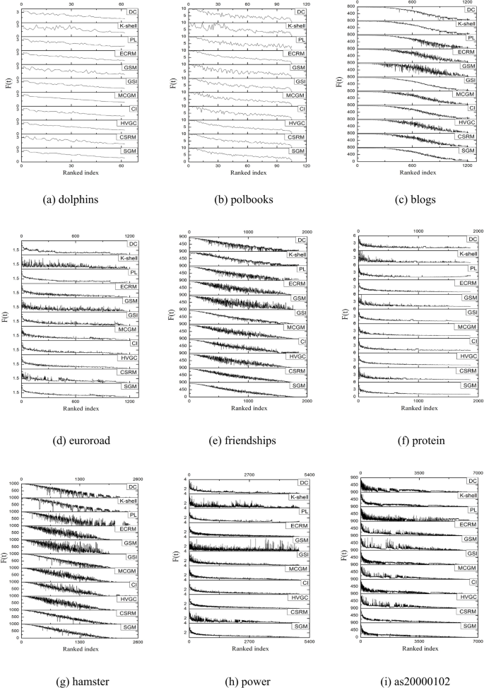
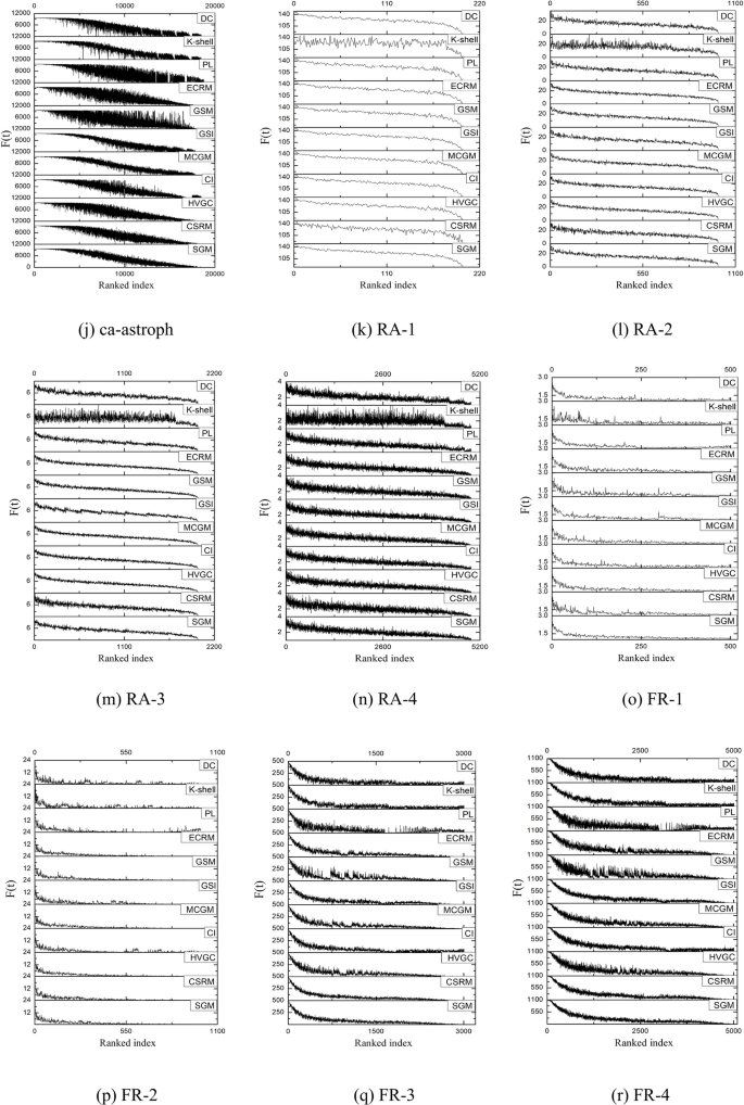
Stacked graphs of 11 algorithms on 18 datasets.
As depicted in Fig. 6, all the algorithms display an overall decreasing trend in their curves. However, algorithms with smoother and less fluctuating curves demonstrate closer alignment with the actual contagion dynamics. Specifically, on networks such as friendships, SGM showcases the fewest small spikes and exhibits smoother waveforms compared to other algorithms, indicating optimal performance on the network. On the hamster, as20000102, FR-3, and FR-4 datasets, both SGM and CSRM demonstrate superior performance with similar smoothness. On the dolphins, and ca-astroph networks, SGM shows slightly more volatility than the MCGM algorithm, yet it outperform other algorithms in terms of overall performance. Similarly, on the euroroad dataset, SGM and PL algorithms rank the highest, showcasing a consistently decreasing trend and the least number of small fluctuations in the waveforms. Regarding the protein, power, FR-1, FR-2 and four random networks, multiple algorithms, including SGM, demonstrate consistent performance.
Consistency of top-N nodes
Given the significance of the Top-N nodes with the highest influence within a network, Jaccard similarity can serve as a metric to evaluate the consistency of Top-N node selections by diverse algorithms compared to those identified through SIR models. Employing Eq. (23), a comparative analysis of similarity was conducted for 15 networks with over 400 nodes. This analysis involved progressively selecting the top 10 to 100 nodes, with the results depicted in Fig. 7. The proposed SGM algorithm demonstrates high performance across all but two networks, namely as20000102 and RA-2, where it exhibits moderate performance.

Jaccard similarity of Top-N nodes.
Capacity differentiation of nodes
Based on the node ranking results obtained from each method and utilizing Eq. (22), the differentiation values in Table 5 are acquired. Remarkably, the proposed SGM algorithm demonstrates exceptional performance across all eleven networks: dolphins, polbooks, blogs, friendships, power, ca-astroph, RA-1, RA-2, RA-3, RA-4, and FR-3. Even on the seven other networks, although the differentiation values may not be the highest, each exceeds 0.94.
Ablation studies
To assess the significance of each component within the SGM algorithm model, an ablation study was conducted. This involved systematically removing specific components and observing the resulting changes in Kendall’s correlation coefficients. ‘SGM’ refers to the algorithm model proposed in this paper, as defined by Eq. (15) to Eq. (19). ‘R-A’, ‘R-B’, ‘R–C’, ‘R-D’, and ‘R-E’ represent the results obtained after sequentially removing specific components, with each step building upon the previous one.
$$R – A = \sum\limits_{{j \in \zeta_{i} }} {\delta_{i} \left( {\frac{SC(i)SC(j)}{{ds_{i,j}^{2} }}} \right)},$$
(24)
$$R – B = \sum\limits_{{j \in \zeta_{i} }} {\frac{SC(i)SC(j)}{{ds_{i,j}^{2} }}},$$
(25)
$$R – C = \sum\limits_{{j \in \zeta_{i} }} {SC(i)SC(j)},$$
(26)
The following analysis can be derived from Fig. 8:
-
(1)
‘R-A’ represents a modification of ‘SGM’ by removing the average clustering coefficients and the correlation component. As discussed in Section “Shannon gravity model”, this part of the SGM model aims to minimize the impact of neighboring nodes in networks with sparse connections. Introducing the influence of neighboring nodes in such scenarios could potentially hinder the accurate assessment of the target node’s influence. This is further confirmed by the analysis of the ‘R-D’. While ‘SGM’ performs comparably to ‘R-A’ on most non-sparse networks, it shows superior performance on five sparse networks, namely euroroad, protein, power, and FR-1, which are characterized by low edge density and average clustering coefficients. This demonstrates the effectiveness of incorporating \(\eta_{G}\) into the model, particularly in the context of sparse networks.
-
(2)
‘R-B’ further removes the gravitational coefficient \(\delta_{i}\) compared to ‘R-A’. In most networks, the removal of the gravitational coefficient leads to a decrease in the Kendall’s \(\tau\). In artificial random networks, the impact of removing the gravitational coefficient is not significant. This is because random networks are generated with a uniform probability of connection, resulting in the maximum and average k-shell values being very similar. As the gravitational coefficient \(\delta_{i}\) is correlated with the k-shell value, the removal of this component has a relatively insignificant impact on random networks.
-
(3)
‘R–C’ further eliminates the distance dsi,j from the gravity model compared to ‘R-B’. It can be observed that ‘R–C’ has a significantly lesser impact than ‘R-B’ on most networks, highlighting the necessity of this part of the design.
-
(4)
‘R-D’, compared to ‘R–C’, removes the effect of neighboring points SC(j). For most networks, the Kendall’s \(\tau\) appears to decrease. However, in the case of sparse networks such as euroroad, protein, power, FR-1, and FR -2 (which have a low ratio of connected edges to nodes and small average clustering coefficients), ‘R-D’ performs better than ‘R–C’. This suggests that for sparse networks, including the influence of neighboring points leads to poorer results. However, due to the compensation factors in other parts of the model, the proposed SGM algorithm performs very close to or even better than ‘R-D’ on sparse networks.
-
(5)
‘R-E’ differs from ‘R-D’ by removing the logarithmic component of the sum of first-order neighbor degree values of node i, retaining only the degree value component. A significant performance decrease is observed across all 18 networks, underscoring the effectiveness of the Shannon capacity design for nodes.


Experiments on the ablation of SGM algorithmic models.
Case study
In recent years, the global impact of the COVID-19 pandemic has presented significant challenges. This study examines the efficacy of the SGM algorithm using the Epi-1 dataset24, which consists of a network comprising 647 nodes linked by 4645 relational edges. The network’s structure, following modularization, is depicted in Fig. 9. It is noteworthy that, while virus propagation is inherently directional at any given moment, this paper adopts the approach of Shetty et al.24 and considers a scenario where the virus can propagate bidirectionally. Consequently, Epi-1 is treated as an undirected and unweighted network.

COVID-19 network diagram.
It is essential to identify individuals within the network who exert greater influence over the transmission of the virus, thereby curbing the spread of the epidemic. Hence, in this manuscript, the Top-20 nodes for each algorithm’s computational outcomes on Epi-1 are selected to infect other nodes, resulting in the eventual propagation pattern illustrated in Fig. 10 and Table 6. Given the substantial likelihood of COVID-19 transmission, the contagion probability in the simulation ranges widely from 0.05 to 0.5. Among these algorithms, SGM, CSRM, PL, and DC exhibit the most effective and approximate contagion effects. This is attributed to the fact that these four algorithms select essentially the same Top-20 ranked nodes, as shown in Table 7. The infectivity of algorithms such as ECRM, CI, GSI, and HVGC demonstrates a slightly lesser degree of effectiveness. Meanwhile, the algorithms GSM, k-shell, and MCGM are considered to be the least effective. As shown in Table 7, when the probability of contagion is set to 0.1, the Top-7 nodes (3855, 3856, 3857, 3858, 3859, 3860, 3861) identified by the SIR model consistently rank within the Top-20 nodes across all 11 algorithms. Hence, the substantial variance in the ultimate contagion size primarily arises from the notably distinct behavior of the remaining thirteen nodes. For example, in addition to the seven nodes previously mentioned, the remaining 13 nodes within the Top-20 identified by the SGM, CSRM, PL, and DC algorithms are as follows: 3073, 3075, 3079, 3756, 3757, 3758, 3759, 3760, 3916, 3091, 4550, 3176, and 3177. Furthermore, the Kendall’s correlation coefficients of the four algorithms, SGM, CSRM, PL, and DC, which exhibited identical performance in the Top-20 contagion scenario, were compared. The average \(\tau\) values for the SGM, CSRM, PL, and DC algorithms, as the probability of contagion varied from 0.05 to 0.5, were found to be 0.7665, 0.6927, 0.6719, and 0.6727, respectively. These results indicate that SGM outperforms the other three algorithms in terms of Kendall’ correlation. Overall, the SGM algorithm introduced in this study proves proficient in identifying pivotal nodes crucial for propagating the COVID-19 network (Epi-1).

Top-20 node contagion size on Epi-1 networks.
link


