


This paper mainly realizes D2D communication resource allocation technology applied in an embedded system under the background of the multimedia computer. If RIS is deployed in a D2D communication system, the controller is responsible for information interaction with a base station and intelligently controls the phase shift of transmitting elements. By optimizing the beamforming vector and RIS phase shift of the base station, the system security level is improved. The multi-scale parallel CNN model is added to the D2D channel model, and the convolution layer is used to extract the channel state information.
RIS auxiliary D2D communication system
A downlink of RIS-assisted D2D communication system is established. As shown in Fig. 1, the base station is equipped with M antennas, and a CU and K pairs of D2D users are distributed around the base station. Each pair of D2D users includes a D2D transmitter (DT) and a D2D receiver (DR). Considering the actual cost and feasibility, the reflection phase of RIS is taken as a discrete value, in which RIS contains n reflection units. It is assumed that the phase shift of each reflection unit is 2 bit, and the phase shift range is [0, 2π]. In particular, assuming that the channel information state is known, the channel gains from BS to RIS, Cu, Dr, and Eve are respectively \(HBI \in \mathbbC^N \times M,h_BC^H \in \mathbbC^1 \times M,g_BD^H \in \mathbbC^1 \times M,g_BE^ \in \mathbbC^1 \times M\);The channel gains from RIS to Cu, Dr and Eve are\(h_IC^H \in \mathbbC^1 \times N,h_ID^H \in \mathbbC^1 \times N,g_IE^H \in \mathbbC^1 \times N\);The channel gains from DT to RIS, Dr, Cu and Eve are\(h_DI^ \in \mathbbC^N \times 1,h_DTDR^ \in \mathbbC^1 \times 1,g_DC^ \in \mathbbC^1 \times 1,g_DE^H \in \mathbbC^1 \times 1\).

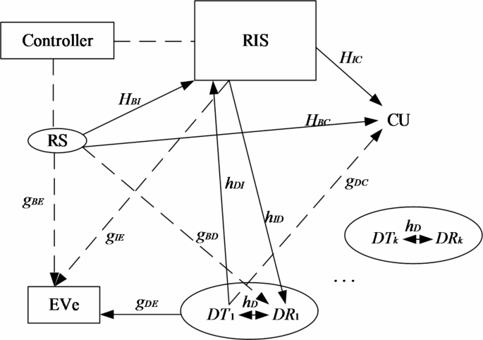
RIS-assisted D2D communication system.
mm-wave D2D channel model
In this paper, Saleh valenzula theoretical channel model18 is adopted, the channel vector is expressed as:
$$hk,m=\sqrt \fracNLk,m \sum\limits_l=0^Lk,m \alpha _k,m^(l) a(\varphi _k,m^(l),\theta _k,m^(l))$$
(1)
Among them,\(Lk,m\)represents the number of multipaths between the m-th sub reflector and the k-th user;\(\alpha _k,m^(l)\)represents the gain of the 1st path;\(\varphi _k,m^(l)\)and\(\theta _k,m^(l)\)Indicates the azimuth and elevation of the i-th path;\(a(\varphi _k,m^(l),\theta _{k,m}^{(l)})\)is the array response vector, which can be expressed as:
$$a(\varphi ,\theta )=aaz\left( \varphi \right) \otimes ael\left( \theta \right)$$
(2)
Where, the horizontal and vertical array response vectors are respectively:
$$aaz\left( \varphi \right)=\frac1\sqrt Ns1 {\left[ {e^\fracj2\pi d1\sin \varphi \lambda } \right]^T},i \in I(Ns1)$$
(3)
$$ael\left( \theta \right)=\frac1\sqrt Ns2 {\left[ {e^\fracj2\pi d2\sin \theta \lambda } \right]^T},j \in I(Ns2)$$
(4)
Among them,\(\lambda\)is the signal wavelength,\(d1\)and\(d2\)are the horizontal and vertical spacing of elements,\(Ns1\)and\(Ns2\)represent Antenna elements in horizontal and vertical directions respectively.
RIS Technology
As a new revolutionary technology, reconfigurable intelligent surface (RIS) can realize the high efficiency of spectrum and energy6. Specifically, RIS is an electromagnetic artificial surface composed of many reflection units, where the phase and amplitude of the incident signal can be adjusted by software programming to improve the signal quality at the receiving end without additional energy consumption. Therefore, RIS can be used to design passive beams, that is, by changing the reflection coefficient of each reflection unit to enhance the required signal and suppress interference. The typical operating architecture of RIS is shown in Fig. 2, which usually consists of an antenna array integrated with many reflectors and a controller. The controller connected with RIS can adjust the reflection coefficient intelligently and communicate with other network components to realize the reconfiguration of wireless communication environment, to improve the anti-interference ability of D2D communication system at the physical layer level.

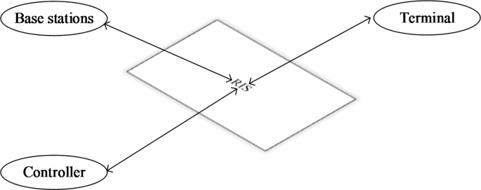
Typical working architecture of RIS.
Multi-scale parallel CNN
To solve the problems of difficult optimization, slow transmission speed and poor security performance in D2D communication system, a multi-scale parallel CNN model is proposed in this paper, as shown in Fig. 3. Firstly, the convolution layer is used to extract the channel state information; Then, the best resource allocation scheme is selected through the full connection layer. The parallel CNN model can not only reduce the complexity of a single model, but also enhance the stability and scalability, which can upgrade the security level of the system while significantly reducing the complexity and running time.

Firstly, a parallel computing model composed of two CNN is constructed, and the specific parameters of each CNN model are set; Then, the outliers far away from the cluster are regarded as outliers and eliminated, and the remaining data samples are normalized to get the required data set, and the data set is divided into a training set and verification set in the ratio of 8:2. Finally, the training set is used to train the model, and the verification set is used to verify the effect of the parallel CNN model.
Model structure
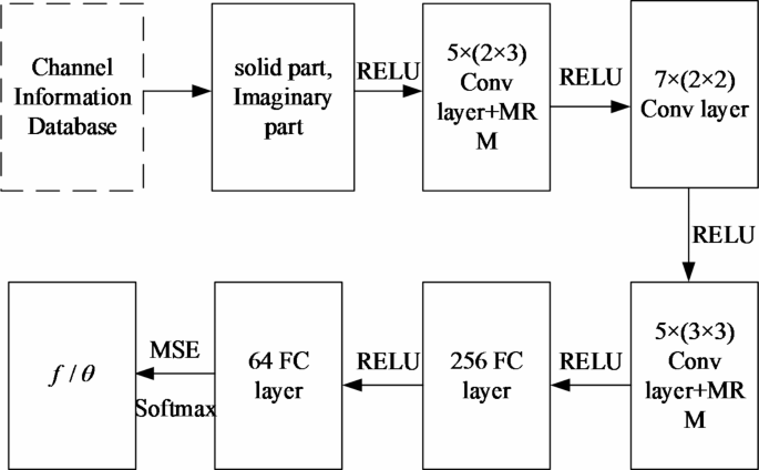
In the multi-scale parallel CNN architecture depicted in Fig. 4, eachCNN is designed with a structured approach to function optimization. The architecture integrates ReLU activation functions and incorporates a multi-scale residual module to enhance both feature extraction and learning capabilities. The ReLU activation function is applied across various stages, including convolutional and pooling layers, to introduce non-linearity. This function outputs the input directly if it is positive; otherwise, it outputs zero. By doing so, ReLU facilitates the network’s ability to learn complex patterns and maintain sparsity in activations, which contributes to computational efficiency and improved convergence rates.
The architecture includes two fully connected layers that play a crucial role in aggregating features and transitioning to a more compact representation. The first fully connected layer consists of 256 neurons, each activated by the ReLU function. This layer serves to condense the high-dimensional feature maps into a flattened representation that is suitable for further processing. The subsequent fully connected layer contains 64 neurons, also utilizing ReLU activation, and further refines the features extracted by the previous layer. This dense layer offers a more compact representation of the learned features, preparing them for the final output stage.
In terms of loss functions, the Mean Squared Error (MSE) is employed in the output layer of the CNN to measure the average squared difference between the predicted values and the actual values. This loss function is particularly suitable for regression tasks where the goal is to minimize the error between the predicted and true continuous values.
Additionally, the Softmax function, although not a loss function per se, is integral to classification tasks within the CNN framework. Softmax converts the output scores (logits) of the final layer into probabilities by exponentiating the logits and normalizing them across all possible classes.
While MSE is conventionally used for regression tasks, classification tasks typically utilize cross-entropy loss in conjunction with the Softmax function. The use of MSE with Softmax might be unconventional unless the network architecture addresses both regression and classification tasks separately. In such cases, different branches of the network may handle regression and classification outputs independently, each utilizing the most appropriate loss function for its specific task.

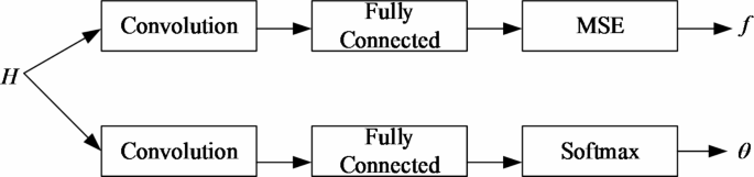
Structure of a single CNN.
A CNN model is used to solve the beamforming vector f, which is constructed as a regression problem. Another CNN model solves the phase shift θ of N reflection units in RIS, which is a classification problem. Specifically, each model consists of the following two parts.
-
(1)
The feature extraction part, which consists of three convolution layers, is responsible for extracting key features from the channel information state.
-
(2)
The resource selection part, which is composed of two fully connected layers, uses the extracted features to select the best resource allocation scheme. Because each CNN in the parallel CNN model can be trained and used independently, the running time will be significantly reduced.
The multi-scale residual module is an advanced architectural component in CNN designed to enhance feature extraction across different scales. This module incorporates residual connections and multi-scale processing, which significantly improves the network’s ability to capture and represent both local and global patterns within the data. Residual connections, which bypass one or more convolutional layers, help address the vanishing gradient problem and enable more effective training of deeper networks. By facilitating the direct passage of input to the output of the block, these connections mitigate degradation issues and ensure smoother gradient flow during backpropagation. Additionally, the multi-scale processing aspect of the module allows the network to learn features from various granularities, aggregating information from multiple convolutional layers. This capability enriches the feature representation, making the network more adept at understanding complex patterns.
The integration of bottleneck residual modules with multi-scale residual modules amplifies the CNN’s capacity for feature extraction. Bottleneck residual modules facilitate the construction of deeper networks with fewer parameters, balancing efficiency and performance. This design approach enables the network to capture complex patterns while reducing computational costs. Combining these modules with standard convolution residual modules enhances the network’s width, allowing for the processing of a broader range of features. This combination not only increases the network’s ability to learn from extensive feature sets but also contributes to improved model performance. Through these enhancements, the multi-scale residual module, in conjunction with bottleneck and convolution residual modules, plays a crucial role in advancing CNN architectures.
In this paper, the multi-scale residual modules added in the first and third convolution layers mainly absorb the multi-scale connection idea of ResNet network, and by combining the bottleneck residual module with the convolution residual module, the width of CNN is enlarged to help the model extract more multi-scale feature information.
AdamW algorithm optimization
After research, it is found that the convergence of the model cannot be effectively guaranteed during training, and there are some problems such as non-convergence or slow convergence. To better deal with the convergence problem of the model, AdamW algorithm19 adds weight attenuation factor when updating parameters w. Generally, other training parameters and methods of 0.01 are the same as Adam’s algorithm. Compared with Adam’s algorithm, AdamW algorithm often has less loss in training set and test set, and also produces better generalization performance when the same training times are carried out.
The AdamW optimization algorithm is an extension of the Adam algorithm, designed to enhance regularization and generalization by integrating weight decay directly into the parameter update rule. The choice of hyper-parameters plays a critical role in achieving effective training and model performance. In this study, a learning rate of 1 × 10⁻⁴ was selected, balancing the need for convergence speed with the risk of overshooting minima. This value is a common default for AdamW and typically requires empirical tuning based on specific datasets and models. 1, set to 0.9, controls the exponential decay rate for the first moment estimates, which represent the moving average of gradients. This value ensures a balance between incorporating past gradient information and adapting to current gradients, thus stabilizing training. Similarly, \(\beta\)2 was chosen as 0.999, which governs the exponential decay rate for the second moment estimates, reflecting the moving average of squared gradients. This setting provides adequate smoothing and stability in gradient variance estimation.
Weight decay \(\lambda\) is another crucial hyper-parameter in AdamW, set to 0.01 in this study. Weight decay functions as a regularization technique that penalizes large weights, thereby mitigating overfitting. This choice, though adjustable, is a typical starting point that aligns with the regularization needs of many models. The epsilon \(\varepsilon\) parameter, set to 1 × 10⁻⁸, ensures numerical stability by preventing division by zero during the parameter update process.
The batch size, set to 32, determines the number of training examples used in each iteration. This value was chosen to strike a balance between computational efficiency and memory constraints. Larger batch sizes could accelerate training but would demand more memory, while smaller sizes might improve generalization. Additionally, the number of epochs, set at 50, represents the total number of passes through the entire dataset. This number provides a reasonable starting point for model training, though it should be monitored and adjusted based on convergence behavior and validation performance.
The training process involves initializing the model parameters and the AdamW optimizer with the specified hyper-parameters. During each training iteration, the forward pass computes the model’s predictions and the loss, followed by a backward pass to calculate gradients. The AdamW update rule then applies the parameter updates, incorporating the weight decay term. Post-iteration, the model’s performance is evaluated on a validation set to monitor for overfitting and convergence.
Training process
Each element of millimeter-wave channel matrix has amplitude and phase, which is transformed according to Euler formula, and each element is expressed as a complex number20. If training with parallel CNN model, it will be difficult to extract features by using complex numbers as input. Therefore, in this paper, the real and imaginary parts of elements are split and spliced into a two-dimensional matrix. According to the system configuration, the input data dimensions of the parallel CNN model are \(\left\ M+N+MN+K^2+K^2N,2 \right\\).
In the training stage, firstly, the network parameters are initialized, the channel information is input into the neural network, and the output is calculated through the network forward propagation. Then, the output result is calculated to get the loss function, the network settings are then updated via back propagation. Finally, the output of the loss function is minimized and tends to be stable, and the training of the CNN model is completed.
In the testing phase, the trained model is evaluated by using the test data set. Firstly, the channel matrix is used as input to train the output parallel CNN model, and then the output results are compared to the traditional algorithm to calculate the prediction accuracy of the parallel CNN model. The specific process is as follows.
-
(1)
Construct a parallel CNN model and divide the data set into training set and testing set.
-
(2)
Weight the neurons in the initial model randomly, and set the learning rate, each batch of input data and training times.
-
(3)
Train the parallel CNN, input the training data, get the output value through forward propagation, calculate the error-by-error function, and use Adam optimizer to optimize the parameters in the network.
-
(4)
Repeat step (3) until the error value is less than the error tolerance or reaches the maximum training times.
-
(5)
Evaluate the performance of parallel CNN model by using verification set.
link