Communication spectrum prediction method based on convolutional gated recurrent unit network

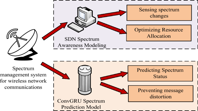
In the rapidly developing field of wireless communications, efficient management of spectrum resources has become a crucial issue. This study conducts an in-depth discussion on spectrum sensing and prediction technology and proposes two innovative model designs: a communication cooperative spectrum sensing model based on channel aliasing dense connection network, and a convolutional gated recurrent neural network based on communication spectrum state prediction model. The overall framework structure diagram of the entire research is shown in Fig. 1.

Overall research framework diagram.

Figure 1 shows the overall framework of this research. This research is mainly divided into two parts, namely building a spectrum sensing model and a spectrum prediction model. These two models are proposed to accurately monitor and predict spectrum usage status to improve the overall utilization efficiency of spectrum resources in wireless communication systems.

Design of spectrum sensing model for communication cooperation based on channel aliasing dense connection network

Spectrum sensing technology refers to sensing and monitoring the usage of radio spectrum in wireless communication systems in order to effectively utilize spectrum resources. Spectrum sensing technology can detect, identify, and monitor idle or underutilized frequency bands in the radio spectrum in real time so that other wireless devices can communicate on these idle frequency bands, thereby improving the operating efficiency of the entire communication system.

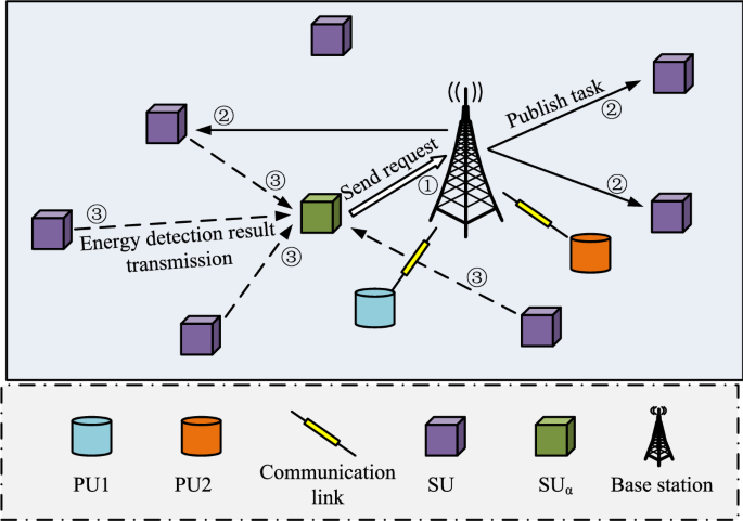
CR is a wireless communication technology. Its core idea is to enable wireless devices to have intelligent cognitive and adaptive capabilities and be able to autonomously perceive, analyze and make decisions on spectrum usage. Non-Orthogonal Multiple Access (NOMA) is also a wireless communication technology used to enable multiple users to communicate simultaneously on the same frequency band²². Traditional wireless communication systems usually use static spectrum allocation, which allocates fixed spectrum resources to each wireless device. However, most spectrum resources are not fully utilized at different times and locations, resulting in a waste of spectrum resources. Based on this background, this research combines CR and NOMA, using CR technology to give the communication system intelligent sensing and decision-making capabilities to more effectively utilize spectrum resources. NOMA technology allows multiple users to communicate on the same site. Non-orthogonal data are transferred on the frequency band. The advantage of Cognitive Radio-Non-Orthogonal Multiple Access (CR-NOMA) technology is that it improves spectrum utilization and system capacity through intelligent sensing and allocation of spectrum resources. At the same time, through the NOMA technology, multiple users can perform parallel data transmission on the same frequency band, providing higher system throughput and user experience. Figure 2 shows the CR-NOMA spectrum sensing model.

Spatial distribution map of the CR-NOMA spectral perception model.

The spatial distribution of the spectrum-aware model under CR-NOMA technique is shown in Fig. 2. In Fig. 2, Primary User (PU) and Secondary User (SU) are not only randomly distributed spatially through different shapes, but also perceive spectrum occupancy through energy detection. Specifically by analyzing the signal strength received by the SU to distinguish the active state (transmitting) and idle state (not transmitting) of the PU to accurately determine the spectrum occupancy. PU1 and PU2 denote two different PUs, respectively. \(\textSU_\texta\) represents the cluster heads. In addition, it is shown in Fig. 2 how to divide the spatial location of the entire enclosed area into an equal area grid and ensure that the location of each SU is in the grid. NOMA is used to connect multiple PUs to the same frequency band and ensure that the transmit power of each PU is constant. 0 and 1 indicate that the PU is currently in idle and operational states, respectively. The spatial location of the entire closed area is divided into \(P \times Q\) equal area networks and ensures that the location \(\left( x_n ,y_n \right)\) of each SU is in the grid. All SUs in space use energy detection to perceive the energy information emitted by PU in the current task frequency band, treating SU as a receiver and PU as a transmitter.

The \(t\)-th sampled signal received by the \(n\)-th SU in the perception gap can be calculated using Eq. (1). Equation (1) is expressed as follows.

where \(s_m\) represents the working state of the \(m\)-th PU at the current moment \(t\), \(\Omega_m\) represents the transmission power of the \(m\)-th PU in its current operating state, \(h_m,n\) represents the channel gain between the \(m\)-th PU and the \(n\)-th SU, \(x_m \left( t \right)\) represents the transmission signal of the \(m\)-th PU, and \(\delta_n \left( t \right)\) represents the Gaussian white noise of the \(n\)-th SU.

The relationship between PU, SU and channel gain can be expressed by Eq. (2), which is shown below.

where \(k\) represents fixed transmission loss, \(d\) represents the distance between the transmitter and receiver, \(\left( x_m ,y_m \right)\) and \(\left( x_n ,y_n \right)\) represent the spatial coordinates of the \(m\)-th PU and the \(n\)-th SU, respectively, and \(a\) represents the path loss index.

From Eq. (2), when the distance between the receiver and the transmitter is farther, the spectrum signal perceived by the SU is weaker. Based on Eq. (2), the formula for the observed value of spectral energy in the sensing gap can be further obtained as shown in Eq. (3).

where \(T\) represents the number of signal samples at the target frequency point, \(e_n\) represents the observed value of spectral energy, and \(\left| y_n \left( t \right) \right|\) represents the modulo operation on the spatial ordinate of the \(n\)-th SU at time \(t\).

Dividing the \(P \times Q\) equal-area network based on spatial location, the cluster head will express the energy observations of each SU combined with the location information in the form of a matrix. Equation (4) is utilized to represent the matrix, which is expressed as follows.

where \(E_PQ\) represents the spatial spectrum energy observation matrix and \(e_PQ\) represents the energy observation values possessed by each grid in the matrix.

The exact value of \(e_PQ\) is calculated using Eq. (5), which is shown below.

where there is no SU in grid \(P \times Q\), \(e_PQ = 0\), and on the contrary \(e_PQ = e_n\).

Through Eqs. (1) to (5), the gray scale map of the perceived energy observation matrix in a certain space can be obtained, so that the positional change of SU and PU as well as the working status can be concluded.

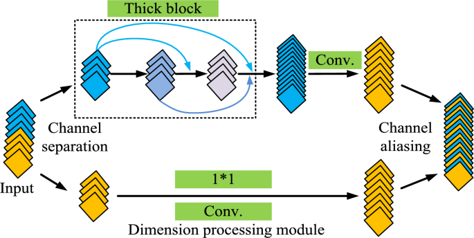
To further identify the grayscale map of the sensed energy observation matrix, the study proposes a communication collaborative spectrum sensed energy identification model using Shuffle Dense Network (SDN), which is a combination of channel shuffle and densely connected convolutional networks. Channel Shuffle is a technique used in CNN that aims to improve cross-channel correlation of features and network performance while maintaining computational efficiency by redistributing channels between different convolutional layers. Densely connected convolutional network is a network architecture where each layer is directly connected to the other layers of its own network. And each layer is directly connected to the other layers of its own network before it. This densely connected structure facilitates more efficient transfer of information and gradients and can reduce the number of parameters in the model. SDN is composed of Shuffle Dense Block (SDB) and the basic structure of SDB is shown in Fig. 3.

Structural diagram of SDB.

Figure 3 shows the basic structure of SDB. It is used to enhance channel coding performance in communication systems, mainly composed of input buffer, aliaser, and output buffer. Aliaser is a core part of SDB, mainly responsible for rearranging input data blocks to increase the spacing and correlation between data, and provide better error correction performance. Aliaser usually adopts different aliasing modes or algorithms, such as block aliasing, bit aliasing, interleaver, etc. The input cache is used to temporarily store input data blocks and wait for aliaser processing. The size and structure of the input cache usually match the working mode and requirements of aliaser. The output cache is used to store the data blocks output by the aliaser. The size of the output cache usually matches the size of the input cache to ensure the correctness and integrity of data during the aliasing process. After inputting the image into it, SDB will perform channel segmentation on the feature map, dividing it into two equal parts. After different feature extraction, the two feature maps are finally merged.

In order to avoid feature disappearance and insufficient feature transfer during the feature transfer process, the study used multiple SDBs and channel aliasing technology to build the final SDN for identifying the grayscale image of the perceptual energy observation matrix²³. The operation flow chart of SDN is shown in Fig. 4.

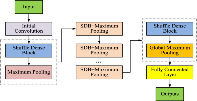
Flow chart of SDN operation.

Figure 4 shows the operation flowchart of SDN, which shows that the final constructed SDN is composed of multiple SDB modules connected in series. In addition, Fig. 4 shows the operation flow of DN in detail. It is mainly divided into spectrum data input, initialization processing, convolution operation to extract signal features, pooling operation to reduce the size of the feature map to remove redundant information, global maximum pooling for feature dimensionalization, fully-connected layer for feature classification, and outputting the determination results of spectrum occupancy. Firstly, spectrum data are input. Then the data are initialized and convolution operation is performed. Next, a maximum pooling layer with a dimension of 2*2 and a step size of 2 is added behind each SDB module. It is used to reduce the size of the feature maps in the channel and remove redundancy and improve the computational speed of the model and avoid overfitting of the model training. Then a global maximum pooling layer is added behind the last SDB module, whose purpose is to fit the output features according to the number of channels. So the dimensionality reduction of the output features can be realized and the classification of the features can be facilitated by the final fully connected layer²⁴. Finally, the features after the fully connected layer are categorized and output.

Communication spectrum state prediction model design based on convolutional gated RNN

Spectrum prediction in CR scenarios can predict spectrum occupancy in advance and improve spectrum reuse efficiency^25,26. Since spectrum occupancy has a strong correlation in time, deep neural network models based on extracting time-series spectrum features are widely used. However, most current models are limited to two-dimensional features in the frequency domain and time domain, ignoring the spatial domain features, or only single-step prediction, and the prediction results have certain limitations. This chapter proposes a prediction scheme based on the Convolutional Gated Recurrent Unit (ConvGRU) network, which combines three-dimensional features of time, space, and frequency for multi-slot long-term spectrum prediction, aiming to improve the prediction performance of the current spectrum prediction model. The spatial distribution structure of the spectrum prediction system is shown in Fig. 5.

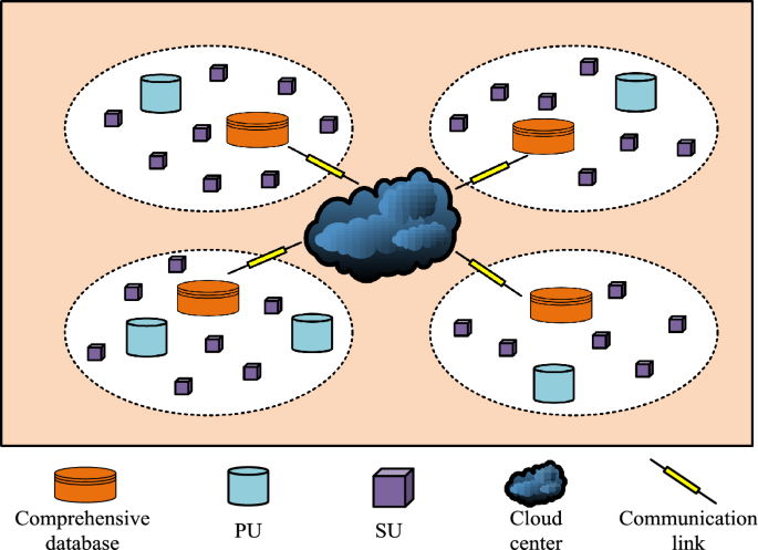
Spatial distribution map of the spectrum prediction model.

The spatial distribution of the spectrum prediction system model is shown in Fig. 5. The whole space contains PUs, SUs, databases, cloud processing centers, and communication links, which are represented by different graphics. PUs and SUs are randomly distributed in the whole space. The whole space is divided into several small parts and a spectrum information database is deployed in each part. Finally, the cloud center is used to connect the paWhen the sensing task arrives, SU is able to perform spectrum sensing, which can be represented by Eqs. (6) and (7). Firstly, the value of the signal received by the SU participating in the sensing task is calculated as shown in Eq. (6).

where \(y_ij \left( n \right)\) represents the signal received by the \(i\)-th SU participating in the perception task \(j\), \(\delta_i \left( n \right)\) represents a mean of 0, \(x_ij \left( n \right)\) represents the useful signal received by the \(i\)-th SU participating in the perception task \(j\), and \(H_0\) and \(H_1\) respectively indicate that the spectrum is in an idle state and in use state.

After calculating \(y_ij \left( n \right)\), the equation for \(x_ij \left( n \right)\) is then obtained as shown in Eq. (7).

where \(s_j \left( n \right)\) represents the transmission signal of the \(j\)-th PU and \(h_ij \left( n \right)\) represents the channel coefficient between the \(i\)-th SU and the \(j\)-th PU.

SU not only performs the sensing task by performing energy superposition with multiple signal samples, but also uses these samples to identify false occupancy situations. By analyzing the statistical properties of the energy superposition values, it is possible to distinguish between real spectrum occupancy and pseudo-occupancy signals caused by environmental noise or other non-occupancy sources. The number of times each SU samples the signal from the PU during the perception time slot is denoted as \(S\). The SU performs energy superposition by multiple signal sampling, which is calculated as shown in Eq. (8).

where \(E_ij\) represents the energy superposition value.

Due to the distance between SU and PU in practical applications, it is necessary to set a decision gate to verify their status. The sensed data will be sent to the cloud center in the form of time-series spectrum between different communities. Then data integration will be carried out by the cloud center^27,28. By filling in the matrix block, the specific situation of the temporal spectrum occupying the image can be obtained. Then, ConvGRU is used for spectrum prediction, and spectrum sensing tasks and spectrum resources are allocated based on the prediction results. The operation flow of the spectrum prediction algorithm is shown in Fig. 6.

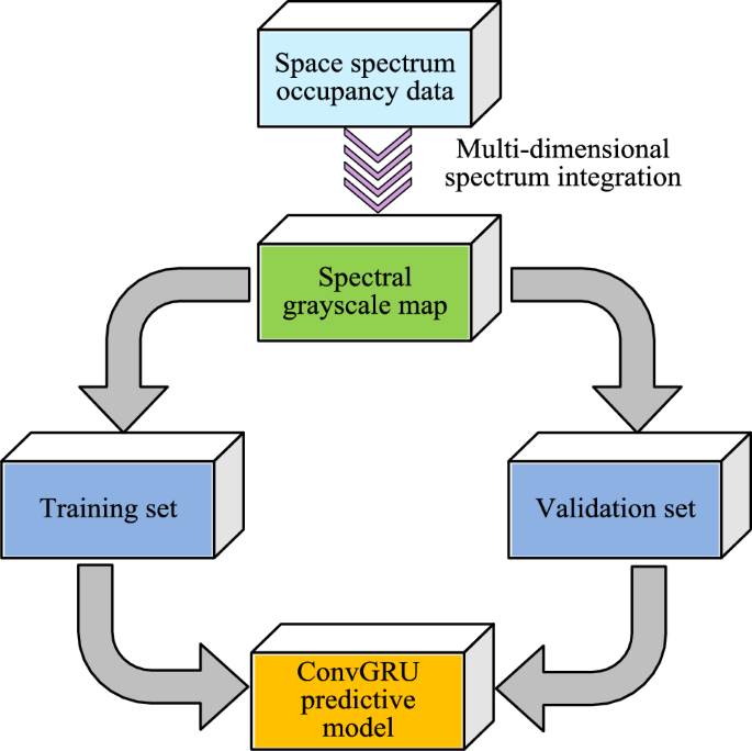
Flow chart of spectrum prediction.

The operation flow chart of the spectrum prediction algorithm is shown in Fig. 6. From Fig. 6, the whole spectrum prediction can be divided into two parts: data preprocessing and model building. It exhaustively depicts the complete operation flow of the ConvGRU prediction model, from data preprocessing to the output of final prediction results. In the data preprocessing stage, the spatial spectrum occupancy data are first integrated multidimensionally to generate the time-series spectrum grayscale map. Next, when building the model, the preprocessed data are analyzed using ConvGRU. The model places special emphasis on the extraction of spatio-temporal features, and each ConvGRU unit is able to integrate the information of current and historical frames. Eventually, the model combines all the extracted features for prediction and outputs the future state of spectrum occupancy. By integrating multidimensional spectral features, not only can the input features of the network be increased, but also the prediction accuracy of the ConvGRU prediction model can be further improved. The feature extraction process of ConvGRU prediction model is shown in Fig. 7.

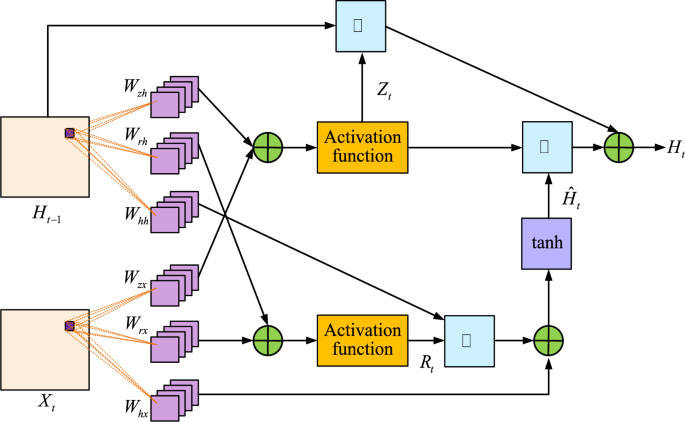
Feature extraction unit plot of the ConvGRU prediction model.

Figure 7 shows the feature extraction unit diagram of the ConvGRU prediction model. The ConvGRU prediction model constructed mainly includes two parts: spatial feature extraction and temporal feature extraction. When each frame of image is input into the network, it is first necessary to extract the spatial features of each input image through the built-in convolutional kernel in the ConvGRU unit. Secondly, the extracted spatial features are transmitted over time and used as input for the next ConvGRU unit. Finally, the output content of each unit in ConvGRU includes both the input features of the current unit and the output features of the historical unit²⁹.

The specific extraction steps of spatial features are shown in Eqs. (9) to (12). Firstly, the value of ConvGRU update gate is calculated as shown in Eq. (9).

where \(X_t\) is the input image of the current unit, \(H_t – 1\) represents the output feature of the previous unit, \(R_t\) represents the reset gate of ConvGRU, \(W_rh\) represents the convolutional kernel that extracts the output features of the previous unit from the reset gate, \(W_rx\) represents the convolutional kernel that extracts the input features of the current unit from the reset gate, \(b\) represents the offset of the current convolutional layer, \(\sigma\) stands for activation function, and \(*\) represents the convolution operation.

The formula for calculating the ConvGRU update gate output value is shown in Eq. (10).

where \(Z_t\) represents the update gate output, \(W_zh\) represents the convolutional kernel used by the update gate to extract historical output features, and \(W_zx\) represents the convolutional kernel used by the update gate to extract the current input feature.

The sigmoid function is selected as activation function, and this activation function is used to set the reset gate output between [0, 1]. When the reset gate approaches 0, it indicates that the historical output features have a smaller impact on the hidden state of the current unit, which is more conducive to long-term prediction³⁰. On the contrary, the reset gate approaches 1 closer, the short-term expectations are more favorable. The implicit state of the current unit is set to \(\hatH_t\) in Eq. (11).

where \(W_hh\) represents the convolutional kernel for extracting historical output features in the hidden state, \(W_hx\) represents the convolutional kernel that extracts the current input feature in the hidden state, \(\tanh\) is the hyperbolic tangent activation function, and \(\circ\) is the Hadamard product.

The final output values of the spatial features in the ConvGRU network are shown in Eq. (12).

Equation (12) shows the calculation formula for the current unit output.

The specific output value of the current unit can be calculated through Eqs. (9) to (12). Figure 8 shows the final designed ConvGRU prediction network structure.

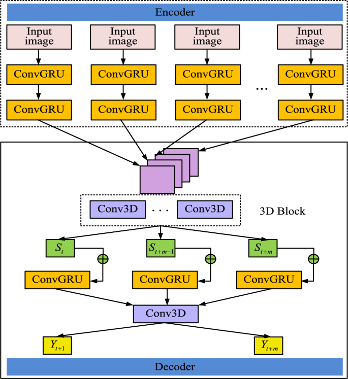
ConvGRU predicted network structure diagram.

The structure of the final designed ConvGRU prediction network is shown in Fig. 8. From Fig. 8, the entire spectrum prediction network structure mainly consists of an encoder and a decoder. In the encoder layer, it consists of two layers of ConvGRU units, and the output of each ConvGRU unit contains the input features of all previous frames. In the decoder layer, to avoid the excessive prediction error, the input sequence \(\left\ H_t – n , \cdots ,H_t \right\\) is used as the input to the decoder, and then all the input features are integrated through the 3D Block layer.

The 3D Block layer contains several Conv3D sub-modules that not only extract features in the time dimension, but also capture subtle changes in channel conditions. Changes in channel conditions, such as signal fading and interference, directly affect the reliability of the signal and the accuracy of spectrum perception. Therefore, the constructed model is able to predict spectrum occupancy more accurately and improve the success rate of spectrum sensing by analyzing these temporal features. The formula for feature extraction using 3D Block layer is shown in Eq. (13).

where \(W_st\) represents the convolutional kernel used by convolutional 3D submodule in 3D block that outputs \(S_t\) to extract features and \(g\left( \cdot \right)\) is activation function.

The most effective prediction information can be extracted by integrating all the feature information, which is used as the input to the prediction layer of the decoder to obtain the final prediction result. The formula for the final prediction result is shown in Eq. (14).

where \(Y_t + 1\) represents the prediction result of \(t + 1\) frames and \(cg\left( \cdot \right)\) represents the nonlinear transformation of ConvGRU units.